Oracle unveils fruits of Project Fusion

After four years since its inception, Project Fusion, Oracle’s next generation suite of enterprise applications will finally be ready to enterprises in 2010.
At the closing keynote of this year’s Openworld conference which saw about 50,000 attendees throng the city of San Francisco, Oracle CEO Larry Ellison said the code base for the Fusion applications is ready, and customers have begun testing the products.
According to Ellison, Oracle will continue to support J.D Edwards and PeopleSoft applications under its Applications Unlimited program, along with its lifetime support policy.
The first version of the brand new Fusion Applications, built from the ground-up with its own technologies and those acquired from other companies, will include Financial Management, Human Capital Management, Sales and Marketing, Supply Chain Management, Project Portfolio Management, Procurement Management as well as Governance, Risk and Compliance.
In addition, enterprises using existing Oracle applications can also augment their software with new applications. These include Distributed Order Management, Customer Data Hub and Talent Management, among others.
Built with a service-oriented architecture in mind, Fusion applications and their underlying components can connect with other applications to pass on data in business processes that span across various lines of business. The software components are all built in Java and can run on industry standard Java middleware.
Business intelligence is also built into the applications for the first time. During a demo, Oracle executives showed a new user interface that notifies IT if something goes wrong with information about what needs to be done to fix a problem, how to do it and possible colleagues to contact for help.
Interestingly, the new Fusion applications are also ready for deployment on the cloud in the form of a SaaS (software as a service) application. However, it is uncertain how Oracle will help companies with the operational processes that need to be undertaken to perform a migration of their software and data to the cloud.

Market Analysis for Business Intelligence OLAP Tools

This graph illustrates the OLAP Product Market Trends from 2000 to 2006, as published in 2007; however, the data does not account for the market consolidations which occurred in 2007, the effects of which are discussed in the first section above.

Business Intelligence OLAP Vendors are ranked and not their individual products, it should be noted that many of the vendors supply multiple OLAP products and applications. Calculating OLAP market shares is quite an involved process, and these figures include OLAP server and client software, applications and OLAP consulting, whether performed by the software author or third-parties. The resulting estimates for the top ten OLAP vendors are shown above.

As the Oracle acquisition of Hyperion did not occur until 2007, it did not change the 2006 or earlier figures, but from 2007, Hyperion’s share will be merged with Oracle’s (which was previously rather low). The joint share will show a declining trend, as both companies separately had declining OLAP market shares, though in absolute terms, it will push Oracle into a stronger second rank behind Microsoft, from its previous weak tenth position.

It took many years for Microsoft SQL Server to establish credibility in the enterprise relational database management system (RDBMS) market; conversely, it has taken much less time for Microsoft SQL Server Analysis Services to achieve the leading position in the OLAP market place. The OLAP Report, announced in 2002 that Microsoft SQL Server 2000 Analysis Services the market leader and has continued to increase that market share year on year.

Examining the graph above you can see that, Microsoft claimed 31.6 percent of the OLAP market in 2006, with Hyperion grabbing 18.9 percent of the market, and Cognos coming in at 12.9 percent. The rest of the vendors held less than a 10 percent market share respectively. The second and third vendors accounted for 31.8 percent of the market, showing that Microsoft has almost double the market of its nearest competitors.

Microsoft is the only major database vendor to have a significant portion of the OLAP market. Oracle had 2.8 percent of the market which lead them to acquire Hyperion in 2007 to improve their overall standings, and IBM only captured 2.2 percent of the market. Both Oracle and IBM have been continually losing market share, however Microsoft gained in the markets overall installations.

Long term, Business Intelligence will play a major role in the competitive position of the major database vendors. The ultimate purpose of Business Intelligence—whether you're using OLAP, data mining, or an old-fashioned spreadsheet—is to help users and companies make better decisions. So, it stands to reason that almost all companies should be using data analytics (or BI) in some capacity.

Lean Execution for JD Edwards™

Utilizing core Oracle JD Edwards Enterprise Software along with Lean Execution™ methodology will empower any enterprise to create a “paperless and information rich environment,” and gain immediate benefits such as:

• Reduction of enterprise cycle times
• Reduction of order lead time
• Reduction of indirect labor costs
• Reduction of direct labor costs
• Reduction of data entry time
• Reduction or elimination of paperwork
• Reduction of work in process (WIP) inventory
• Increase in equipment utilization

Implementing Lean Execution™ techniques enables critical information to flow throughout the organization—including the often-forgotten areas of distribution and manufacturing. This requires that the information is within the control of those who actually produce your goods or services. “Paperless and information rich environments” have been created for a few forward-thinking enterprises, producing dramatic gains throughout their entire organizations. Now you will learn how the same results are possible for your enterprise.

A Lean Execution™ Implementation may employ some of all of the following techniques:.

• THEORY OF CONSTRAINTS
• LEAN THINKING
• JUST IN TIME
• FLEXIBLE MANUFACTURING SYSTEM
• ADVANCED PLANNING & SCHEDULING
• TOTAL QUALITY
• SIX SIGMA
• DEMAND FLOW TECHNIQUES

Our consultants understand the complexities of Modern Enterprises and will follow each possible method through the Planning, Organizing, Scheduling, Directing and Controlling of each implementation. We will assure the most beneficial outcome is achieved in each and every implementation.

Multifacility Planning

In a multifacility operation, planned orders at the demand facility are the source of demand at the supply facility. You set up and maintain multifacility plans to:
Manage the movement of material through distribution networks and multiple production facilities.
Formalize the process of transferring items among your facilities.
Create internal transfer orders to help ensure traceability of materials and their costs between facilities.
Ensure that the facility from which you are ordering has enough inventory in stock to fill the order or schedule the supply plant to produce it.
Schedule production according to realistic time frames.
Use assembly lines at one plant to begin the assembly of a product and a different plant for final assembly.
Handle all resupply movements throughout the manufacturing network.
Multifacility plans allow greater control of your enterprise. You can define facility relationships at any level of detail for an entire facility, a product group, master planning family, or an individual item number. In addition, you can incorporate all your facilities into a single plan.
In Material Requirements Planning (MRP), the system transfers items among your manufacturing plants at the component level. The system transfers component items by generating:
Purchase orders at the demand plant for the supply plant
Sales orders from the demand plant at the supply plant
In the following example, the demand plant (M55) receives components from three different supply plants. Supply plants can also manufacture the end deliverable item.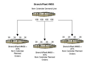

Setting Up Multifacility Planning

You set up multifacility planning to track supply, demand, and movement of material among the individual facilities of your enterprise. Multifacility planning provides a flexible method for planning supply and resupply activities.
In multifacility planning, you must set up a table of supply and demand relationships among your facilities. The system uses these relationships to generate and maintain multifacility plans.

Setting Up Supply and Demand Relationships

Use Branch Relationships Revisions (P3403T) to set up supply and demand relationships for any level of detail that you choose, including:

• Branch/plant
• Product group
• Master planning family
• Individual item number

This approach allows you to maintain supply and demand relationships in one central location, and reduce inventory errors caused by complex facility relationships. In addition, when you set up supply and demand relationships, you can use the following optional features:

Markup
You can have the system automatically mark up the cost of an item when you create a transfer order. The system can adjust the cost by a fixed amount or percentage.
Availability checking
You can ensure that the branch from which you are ordering has enough inventory in stock to fill the order. If the required quantity is not available, the system checks subsequent facilities in the sequence that you define.
Effectivity dates
Use effectivity dates to control the demands that are placed on your supply branches. If an effectivity date that was assigned to a supply branch has expired, the system checks for another facility.
The Material Requirements Planning (MRP), Distribution Requirements Planning (DRP), and Master Production Scheduling (MPS) versions of the Branch Relationships Revisions program use the same processing options. You can vary the settings in the processing options to accommodate the different requirements for a material requirements plan.
Caution
When you delete a supply and demand relationship, the system deletes the entire record.
To set up supply and demand relationships
From the Multi-Facility Setup menu (G3443), choose Branch Relationships Revisions.

1. On Work With Branch Relationships, complete one of the following fields:

• Supply Branch/Plant
• Demand Branch/Plant
• Use the View menu to switch from viewing the supply branch/plant to viewing the demand branch/plant. A processing option controls which branch/plant is the default.

2. To narrow your search, complete one of the following fields and click Find. Enter an item number to display all branch/plants that either supply or demand a certain part. Enter the planning family to display all branch/plants that either supply or demand parts that belong to a specific master planning family.

• Planning Family
• Item Number

3. Choose the record and click Select.
4. On Branch Relationship Revisions, complete the following fields:
Include/ Exclude
Some parts might come from certain branch/plants. In multifacility planning, if Exclude is selected, then the item is supplied by the demand branch only.
Effective From
This date defaults in from the bill of material.
Source Percent
The percent of demand to be supplied by the source branch/plant.
Percent To Fill
This amount of the source percent must be available to be filled by this branch/plant. The percent of demand should be filled to place a transfer order message. A transfer order is generated if Availability Check is on.
5. Complete the following optional fields, then click OK:
Branch Level
The branch that will go first, second, and so on. The lowest level is processed first (the highest numerical value). Ensure all demand is generated before supply is allocated.
Branch Priority
This field shows the sequence within a level branch/plant where requirements are processed.
Transfer Leadtime
This field shows the time to ship the item from the supply to the demand branch plant in days.
Availability Check
If availability check is on, the system checks the availability of the supply branch inventory only. The available balance is committed until a zero inventory balance, and then moves to another supply branch or creates an order in the demand branch.
If availability check is off, then the inventory balance can go negative.

Processing Options for Branch Relationships Revisions (P3403T)
Defaults
Enter the default Branch Relationship display mode.
1. 'D' = Demand branch 'S' = Supply branch
Enter a '1' to automatically update the Branch Level field.
2. Branch Level update

Note
You must set this processing option to ensure that the level of the component branch is one level higher than the header for the source branch. The branch level on the Defaults tab, along with the branch priority, determines the sequence in which the system processes supply and demand plants. The system processes the branches with the highest numerical branch levels first.
Reviewing Branch Relationships
Use the Branch Relationships Chart (P34031) to review supply and demand relationships in a graphical, hierarchical format. The Branch Relationships Chart displays the following:
Branch
Level of the branch
Supply branches for the corresponding demand branch
The Material Requirements Planning (MRP), Distribution Requirements Planning (DRP), and Master Production Scheduling (MPS) versions of the Branch Relationships Chart program use the same processing options. You can vary the settings in the processing options to accommodate the different requirements for a material requirements plan.
To review branch relationships
From Multi-Facility Setup (G3443), choose Branch Relationships Chart.
1. On Work With Branch Relationships Hierarchy, complete the following field to locate the branch/plant for which you want to display supply and demand relationships:
Supply Branch
2. To narrow your search to a specific level of detail, complete one of the following optional fields and then click Find:
Item Number
Plan Family
3. On Work With Branch Relationships Hierarchy, choose a row and click Select to review the branch relationships.


Transfer Orders and Multifacility Planning
Transfer orders are used by the Multifacility Planning system to transfer inventory between branch/plants within your company. The transfer of inventory is done by generating a purchase order at the demand plant and a sales order at the supply plant.
Instead of manually entering the transfer orders, you run Master Planning Schedule – Multiple Plant (R3483), which generates the plan and respective planning messages. You then process the messages.
When the system creates a transfer order from a planning message, the system does the following:
Creates a purchase order for the supply branch/plant that ships the items
Creates a sales order for the demand branch/plant that receives the items
Processes the inventory amounts on the transfer order as a formal purchase and sale of goods
Creates documents—such as orders, pick slips and invoices—that are necessary to complete the transfer
When the sales order is generated, the system uses the Customer Master for certain defaults and validation. The system might check the following settings:
availability checking
partial shipments allowed
default carrier
order holds
freight charges
Markups can also be applied by setting up the Branch Relationships Master File table (F3403).
When the purchase order is generated, the system uses the supplier master to get defaults and validation. The system might check the following settings:
order holds
print messages
landed costs
JD Edwards EnterpriseOne software has standard document types set up for transfer orders. Sales orders use document type ST and purchase orders use OT. These document types are defined in user defined code (UDC) table 00/DT. Thus, you can create your own document types. For example, transfers that are generated by planning might use the ST/OT document types; orders generated manually use alternate document types. Along with the visible difference in document type, the use of different document types allows for differences in accounting, approvals, and order activity rules.
Customer and Supplier Masters and Multifacility Planning

To create transfer orders in the Multifacility Planning system, you are required to set up default customer and supplier masters for the branch/plants that are used.

Note
Transfer orders use the customer and supplier masters in unique ways during order generation.
A customer master is required for the demand plant, and a supplier master is required for the supply plant.
A standard sales order uses the customer address book number for the billing instructions. The sales order that is created for a transfer order uses the address number of the branch from which you are shipping.
A standard purchase order uses the supplier’s address book number. The purchase order that is created for a transfer order uses the address book number of the branch that is receiving the product.
Generating Multifacility Plans
Use one of the following navigations:
From the Multi-Facility Planning menu (G3423), choose MPS Regeneration.
From the Multi-Facility Planning menu (G3423), choose MRP Regeneration.
After you have set up the supply and demand relationships among your branch/plants, you can use the Distribution Requirements Planning (DRP), Master Production Scheduling (MPS), and Material Requirements Planning (MRP) gross regeneration versions of Master Planning Schedule – Multiple Plant (R3483) to generate a multifacility plan. Alternatively, you can use the DRP, MPS, and MRP net change versions of Master Planning Schedule – Multiple Plant to generate a multifacility plan.
When you generate a multifacility plan, the system evaluates selected information, performs calculations, and recommends a time-phased plan for all selected items.
Prerequisite
q Set up DRP/MPS multifacility planning.

Processing Options for Master Planning Schedule – Multiple Plant (R3483)
Horizon Tab
These processing options specify dates and time periods that the program uses when it creates the plan.
1. Generation Start Date
Use this processing option to specify the date for starting the planning process. This date is also the beginning of the planning horizon.
2. Past Due Periods
3. Planning Horizon Periods
Number of planning days
Use this processing option to specify the number of days from the horizon start date for which you want to see daily planning data.
Number of planning weeks
Use this processing option to specify the number of weeks for which you want to see weekly planning data, following the daily data.
Number of planning months
Use this processing option to specify the number of months for which you want to see monthly planning data, following the weekly data.
Parameters Tab
Use these processing options to define processing criteria. The following information concerns your choice of generation type:
Generation Type 1, single-level MPS/DRP. You can use this generation type either in a distribution environment for purchased parts with no parent-to-component relationship, or in a manufacturing environment with parent-to-component relationships. When you use this generation type, the system performs the following actions:
Produces a time series for each item that you specify in the data selection with a Planning Code of 1 on the Plant Manufacturing Data tab of the Work with Item Branch form. This code indicates whether the item is manufactured or purchased.
Does not explode demand down to the components for manufactured items. Use generation type 1 if you first want to process only the master-scheduled end-items. Thus, you can stabilize the schedule before placing demand on the components.
Does not create pegging records.
Generation Type 3, multilevel MPS. This generation type is an alternative to generation type 1 and performs a complete top-to-bottom processing of master-scheduled items. For all parent items that you specify in the data selection, the program explodes demand down to the components. You must specify all of the items to be processed in the data selection, not just the parent items. The program also creates pegging records.
Generation Type 4, MRP with or without MPS. This generation type performs the same functions as generation type 3. After you perform a complete generation and stabilize your master schedule, you can limit data selection to MRP items (with planning codes of 2 or 3), thereby reducing processing time. This action is possible because the system still stores demand from the master-scheduled items in the MPS/MRP/DRP Lower Level Requirements File table (F3412).
Generation Type 5, MRP with frozen MPS. This generation type freezes the master schedule after it has been stabilized. Before using this generation type, make all necessary adjustments to master-scheduled items and release orders to provide supply for the demand. This generation type freezes the entire planning horizon, which is similar to the way the freeze fence freezes a part of the horizon. Running this generation type produces the following results, which apply to MPS items only:
No new orders will be planned.
No messages for existing orders will be created.
The adjusted ending available quantity can be negative.
Demand is only exploded down to components from existing work orders. No -PWO demand from parent items exists; only -FWO demand exists.
1. Generation Mode
1 = net change
2 = gross regeneration
A gross regeneration includes every item specified in the data selection. A net change includes only those items in the data selection that have changed since the last time you ran the program.
Valid values are:
1 net change
2 gross regeneration
2. Generation Type
1 = single level MPS/DRP
3 = multi-level MPS
4 = MRP with or without MPS
5 = MRP with frozen MPS
Please see the help for the Parameters tab for detailed information.
Valid values are:
1 single-level MPS/DRP
3 multi-level MPS
4 MRP with or without MPS
5 MRP with frozen MPS
3. UDC Type
Use this processing option to specify the UDC table (system 34) that contains the list of quantity types to be calculated and written to the Time Series table (F3413). Default = QT.
4. Version of Supply/Demand Inclusion Rules

Use this processing option to define which version of supply/demand inclusion rules the program reads. These rules define the criteria used to select orders for processing.

On-Hand Tab
These processing options define how the program calculates on-hand inventory.
1. Include Lot Expiration Dates
blank = do not include
1 = include
Use this processing option to specify whether the system considers lot expiration dates when calculating on-hand inventory. For example, if you have 200 on-hand with an expiration date of August 31, 2005, and you need 200 on September 1, 2005, the program does not recognize the expired lot and creates a message to order or manufacture more of the item to satisfy demand.
Valid values are:
blank do not consider lot expiration dates when calculating on-hand inventory
1 consider lot expiration dates when calculating on-hand inventory
2. Safety Stock Decrease
blank = do not decrease
1 = decrease
Use this processing option to specify whether to plan based on a beginning available quantity from which the safety stock quantity has been subtracted.
Valid values are:
blank do not decrease
1 decrease
3. Receipt Routing Quantities
Quantity in Transit
blank = do not include in on-hand inventory
1 = include in on-hand inventory
In a manufacturing environment, sometimes it is necessary to establish where stock is, in order to determine whether or not it is available for immediate use. Enter 1 if you want quantities in transit to be included in the Beginning Available calculation on the time series. Otherwise, the program includes these quantities in the In Receipt (+IR) line of the time series. The quantities are still considered available by this program. The difference is only in how you view the quantities in the time series.
Valid values are:
blank do not include in on-hand inventory
1 include in on-hand inventory
Quantity in Inspection
blank = do not include in on-hand inventory
1 = include in on-hand inventory
Use this processing option to specify whether to include quantities in inspection when the system calculates the Beginning Available amount. Otherwise, the system includes these quantities in the In Receipt (+IR) line of the time series. The system still considers the quantities available, but the way in which you view the quantities in the time series differs. Valid values are:
Blank
Do not include quantities in on-hand inventory
1
Include quantities in on-hand inventory
User Defined Quantity 1
blank = do not include in on-hand inventory
1 = include in on-hand inventory

In a manufacturing environment, sometimes it is necessary to establish where stock is, in order to determine whether or not it is available for immediate use. Enter 1 if you want these user defined quantities (defined on Receipt Routings Revisions in the Update Operation 1 field) to be included in the Beginning Available calculation. Otherwise, the program includes these quantities in the In Receipt (+IR) line of the time series. The quantities are still considered available by this program. The difference is only in how you view the quantities in the time series.
Valid values are:
blank do not include in on-hand inventory
1 include in on-hand inventory
User Defined Quantity 2
blank = do not include in on-hand inventory
1 = include in on-hand inventory
In a manufacturing environment, sometimes it is necessary to establish where stock is, in order to determine whether or not it is available for immediate use. Enter 1 if you want these user defined quantities (defined on Receipt Routings Revisions in the Update Operation 2 field) to be included in the Beginning Available calculation. Otherwise, the program includes these quantities in the In Receipt (+IR) line of the time series. The quantities are still considered available by this program. The difference is only in how you view the quantities in the time series.
Valid values are:
blank do not include in on-hand inventory
1 include in on-hand inventory
4. Lot Hold Codes ( up to 5 )
blank = include no held lots in calculation of on-hand inventory
* = include all held lots in calculation of on-hand inventory
Use this processing option to specify the lots to be included in the calculation of on-hand inventory. You can enter a maximum of 5 lot hold codes (41/L). blank include no held lots in calculation of on-hand inventory * include all held lots in calculation of on-hand inventory
5. Include Past Due Rates as a supply
blank = do not include
1 = include
Use this processing option to specify whether the system considers open quantity from past due rate orders as supply. If you enter 1, open quantities from past due rate orders are included in the rate schedule unadjusted (+RSU) line as well as the rate schedule adjusted (+RS) line of the Master Planning Schedule - Multiple Plant program (R3483). Valid values are:
Blank
Do not consider past due orders as supply.
1
Consider past due orders as supply.
Forecasting Tab
These processing options serve the following two purposes:
They determine which forecast types the program reads as demand
They initiate special logic for forecast consumption
1. Forecast Types Used ( up to 5 )
Forecasts are a source of demand. You can create forecasts using 12 different forecast types (34/DF) within the Forecasting system. One is considered the Best Fit (BF) type compared to an item's history of demand. Use this processing option to define which forecast quantities created by which forecast type are included in the planning process. Enter multiple values with no spaces, for example: 0102BF.
2. Forecast Consumption Logic
blank = do not use forecast consumption
1 = use forecast consumption
2 = use forecast consumption by customer
Use this processing option to specify whether the system uses forecast consumption. If you use forecast consumption, any sales order due in the same period as the forecast is included as part of the forecast for that period. The sales order is not considered an additional source of demand. For forecast consumption to be used, the planning fence rule for the item must be H and the planning fence must be 999. You enter these values on the Plant Manufacturing Data form.
Note: When you use forecast consumption, the system applies forecast consumption logic to the aggregate sales order and forecast quantities.
Blank
Do not use forecast consumption.
1
Use forecast consumption.
3. Interplant Demand Consumes Forecast
blank = do not use
1 = use
When using forecast consumption, use this processing option to specify whether to use interplant demand to consume forecast. When using any other planning rule, you can use this option to specify whether to consider interplant demand as customer demand. When the option is set, the system considers interplant demand for firm and planned transfer orders.
When the option is blank, the system ignores interplant demand by forecast consumption or planning rules and considers interplant demand as a separate source of demand. Valid values are:
Blank Do not consider interplant demand as customer demand.
1 Consider interplant demand as customer demand.


Document Types Tab
These processing options establish default document types.
1. Purchase Orders
When you receive messages related to purchase order creation, this document type will appear as the default. The default value is OP.
2. Work Orders
When you receive messages related to work order creation, this document type will appear as the default. The default value is WO.
3. Rate Schedules
When you receive messages related to rate schedule creation, this document type will appear as the default. The default value is AC.


Leadtimes Tab
These processing options let you specify safety leadtimes to allow extra time for delays in receipt or production. Use damper days to filter out unwanted messages.
1. Purchased Item Safety Leadtime
For items with stocking type P, the program adds the value you enter here to the item's level leadtime to calculate the total leadtime.
2. Manufactured Item Safety Leadtime
For items with stocking type M, the program adds the value you enter here to the item's level leadtime to calculate the total leadtime.
3. Expedite Damper Days
Use this processing option to specify the number of days before the system generates an expedite message. If the number of days between the date when the order is actually needed and the due date of the order is less than the number of days entered here, the system does not generate an expedite message.
4. Defer Damper Days
Use this processing option to specify the number of days before the system generates a defer message. If the number of days between the date when the order is actually needed and the due date of the order is less than the number of days entered here, the system does not generate a defer message.
Performance Tab
These processing options define output and specify conditions that might decrease processing time.
1. Clear F3411/F3412/F3413 Tables
blank = do not clear tables
1 = clear tables
Use this processing option with extreme caution! If you enter 1, all records in the MPS/MRP/DRP Message table (F3411), MPS/MRP/DRP Lower Level Requirements (Pegging) table (F3412), and MPS/MRP/DRP Summary (Time Series) (F3413) table are purged.
Access to this program should be limited. If multiple users run this program concurrently with this processing option set to 1, a record lock error results and prevents complete processing.
Valid values are:
blank do not clear tables
1 clear tables
2. Initialize MPS/MRP Print Code
blank = do not initialize the Item Branch file
1 = initialize the Item Branch file
If you enter 1 in this processing option, the program initializes every record in the Item Branch table (F4102) by setting the Item Display Code (MRPD) to blank
If you leave this field blank, processing time is decreased. The system will not clear the records in the Item Branch table (F4102).
Regardless of how you set this processing option, for each item in the data selection the MRPD field is updated as follow:
o 1 if messages were not created
o 2 if messages were created
The Print Master Production Schedule program (R3450) allows you to enter data selection based on the MRPD field.
Valid values are:
blank Do not initialize the Item Branch file.
1 Initialize the Item Branch file.
3. Messages And Time Series For Phantom Items
blank = do not generate
1 = generate
Use this processing option to specify whether the program generates messages and time series for phantom items.
Valid values are:
blank do not generate
1 generate
4. Ending Work Order Status
blank = all messages exploded
Use this processing option to specify the work order status at which messages are no longer exploded to components. If you leave this field blank, all messages are exploded to components.
5. Extend Rate Based Adjustments
blank = do not extend
1 = extend
Use this processing option to specify whether adjustments for rate based items are exploded to components, thereby creating messages for the components.
Valid values are:
blank do not extend
1 extend
6. Closed Rate Status
Use this processing option to specify the status of closed rates. When you plan for a rate-based item, the system does not process rate orders that are at a closed-rate status or a higher status.
Mfg Mode Tab
These processing options specify integration with other systems.
1. Process Planning
blank = discrete
1 = process
If you use process manufacturing, enter 1 to generate the plan based on the forecasts of the co-/by-products for the process. The program then creates messages for the process.
Valid values are:
blank discrete
1 process


Multi-Facility Tab
These processing options define criteria for a multifacility environment.
1. Date Branch
Enter the default branch/plant from which to retrieve the shop floor calendar.
If you leave this field blank, the calendar for each branch/plant is used and processing time increases.
2. Consolidation Method
1 = simple consolidation
2 = branch relationships ( default )
The simple consolidation method (1) adds the supply and demand for each branch, calculates a new time series, and places the result in the consolidated branch specified in the Consolidation Branch processing option.
The branch relationships method (2) uses the Branch Relationships table. This is the default.
Valid values are:
1 simple consolidation
2 branch relationships (default)
3. Consolidation Branch
If your consolidation method is 1 (simple consolidation), enter the branch/plant to contain the consolidated results. If the consolidated branch/plant also contains its own time series data, that data is included in the totals.
4. Category Code
1 = 41/P1
2 = 41/P2
3 = 41/P3
4 = 41/P4
5 = 41/P5
If your consolidation method is 2 (branch relationships), enter the category code of the part that is supplied by one branch/plant to another. There are five user defined category code tables.
Valid values are:
1 41/P1
2 41/P2
3 41/P3
4 41/P4
5 41/P5
5. Manufacture At Origin
blank = create transfer orders for manufactured and purchased items
1 = create transfer orders only for purchased items
Enter 1 if there are manufactured and purchased items in the same category code, but you only want to obtain the purchased items from another branch/plant. Transfer order messages are created for purchased items, and work order messages are created for manufactured items.
Valid values are:
blank create transfer orders for manufactured and purchased items
1 create transfer orders only for purchased items
6. Transfer Order Document Type
blank = OT
When you receive messages related to transfer order creation, this document type will appear as the default. The default value is OT.


Parallel Tab
These processing options specify the number of processors that the system uses during parallel processing. These processing options also specify whether the system runs preprocessing during parallel processing.
1. Number of Subsystem Jobs
0 = Default
Use this processing option to specify the number of subsystems in a server.
The default is 0 (zero).
2. Pre Processing
blank = Do not perform pre processing
1 = Perform pre processing
Use this processing option to specify whether the system runs preprocessing during parallel processing. During preprocessing, the system checks supply and demand and plans only the items within supply and demand. Preprocessing improves performance when you run MRP and is valid only when the number of items actually planned is less than the total number of items in the data selection. Valid values are:
Blank The system does not run preprocessing.
1 The system runs preprocessing.
Working with Multifacility Planning Output

Multifacility planning output consists of information in the time series and transfer order messages. Use the time series information to either accept or override the planning that the system suggests. You should review the transfer order messages for individual item numbers to determine which action, if any, that you need to take.
Reviewing the Time Series for the Multifacility Schedule
To review the multifacility time series
From the Multi-Facility Planning Daily Operations menu (G3414), choose Time Series/ATP Inquiry.
1. On Work With Time Series, complete the following fields and click Find to locate the time series for an item:
Item Number
Branch/Plant
Processing Transfer Order Messages for the Multifacility Schedule
Use MRP/MPS Detail Message Revisions (P3411) to review the transfer order messages for the multifacility schedule. Multifacility scheduling creates messages that are appropriate to the demand and supply facilities. If you process the messages, the system automatically creates transfer orders. You can transfer items between facilities either at cost or at a markup.
To process multifacility transfer order messages
From the Multi-Facility Planning Daily Operations menu (G3414), choose Detail Message Review.
1. On Work With Detail Messages, complete the following fields and click Find to locate the transfer order messages for an item:
Item Number
Demand Branch
2. Choose the transfer order messages that you want to process.
3. From the Row menu, choose Process Message(s) to create the following:
Transfer order for the item
Purchase order number for the demand plant
Sales order number for the supply plant
4. On Work With Detail Messages, review the information for the new orders in the following fields:
Order Number
Start Date
Request Date
Recmd'd Start Date
Recmd'd Complete
Demand Branch
Supply Branch
Multifacility Forecast Consumption
Multifacility forecast consumption in Material Requirements Planning (MRP) is a process to reduce the forecast quantity through the number of sales orders and shipped orders. The goal of forecast consumption is to have your forecast quantity be greater than the total of sales orders and shipped orders. The forecast quantity is consumed either fully or partially. For example, when the sales order quantity is greater than the forecast quantity, then the forecast quantity is fully consumed. The option that you choose is dependent on your need to forecast interplant demand.
Time Series Quantity Types
The system uses the following quantity types (34/QT) for multifacility consumption:
Calculations
If the Interplant Demand processing option for the Master Planning Schedule - Multiple Plant program (R3483) is on, the transfer orders consume the supply plant's forecast. The system does not plan the transfer orders again. The system uses the following calculations when the Interplant Demand processing option is on:
-TIU = (-SOU) + (-ID) + (-FID)
+PLO = (-FSCT) + (-TI)
If the Interplant Demand processing option is off, the system processes the transfer orders as additional demand for the supply plant. The system uses the following calculations when the Interplant Demand processing option is off:
(TIU) = (-SOU)
+PLO = (-FSCT) + (-FID) + (-TI) + (-ID)
Additional Options for Multifacility Forecast Consumption
To have interplant demand consume forecast, you need to add your transfer order type to user defined code (UDC) table 40/CF. The system then accumulates ship-confirmed transfer orders to accumulate in the -SHIP quantity type while still using the orders to consume forecast. Also, regardless of the Interplant Demand processing option, the system processes interplant demand consistently whether the order is planned demand or firm demand. For example, interplant demand either consumes or does not consume forecast.
If you do not want to use the new quantity types, you can make a copy of the 34/QT table with the necessary quantity types. The system completes the calculations but does not display them on the time series. The system displays the following results when you remove the following quantity types:

Introduction to Standard Costing

Standard costing is an important subtopic of manufacturing cost accounting. Standard costs are associated with manufacturing companies and are utilized to manage the costs of direct material, direct labor, and manufacturing overhead.

In lieu of assigning actual or average costs of direct material, direct labor, and manufacturing overhead and rolling these costs into their products, most manufacturers assign a standard cost to their systems. This means that their inventories and cost of goods sold are valued using the standard costs, and not the actual or average costs, of a product. The Manufacturers pays their vendors at actual costs which can vary over time. This results in differences between the actual costs and the standard costs, and those differences are known as variances.

Standard costing and the related variances are valuable to measure the performance of inventory and product production. When a variance arises, management becomes aware that manufacturing costs have differed from the standard (planned, expected) costs.

• If the actual cost is greater than the standard cost the variance is referred to as unfavorable; and unfavorable variances result in the company’s actual profit being less than planned.
• If the actual cost is less than the standard cost the variance is referred to as favorable; and favorable variances result in the company’s actual profit being less planned.
  Timely reporting of these manufacturing variances allows management to take action on the differences from the planned amounts.

This, however, is not the only reason that manufacturers utilize standard costs. In the manufacturing process, materials are issued to work orders and job orders and taken out of the perpetual inventory and show up on the balance sheet on what is known as work in process. Because work in process no longer has any part number identity, it is retained as a gross value on the balance sheet. If a part is issued to a work order and the value of that part is written to the general ledger work in process account at its current value. If the company were using average cost to value their products and the item in question is received at a higher price prior to the work order being completed, then the item will be relieved from inventory in the future at the new value, causing a negative balance in the work in process account. Multiply this by thousands of transactions and you will see why it is important to utilize standard costs in a manufacturing system.

The perpetual inventory is maintained at standard cost (including Direct Materials and Subassemblies), and the standard cost of finished goods becomes the sum of the standard costs of the following values:

• Direct material
• Direct labor
• Manufacturing overhead
• Variable manufacturing overhead
• Fixed manufacturing overhead

Increased Business Value With Collaborative Manufacturing

In today’s emerging global economy, seamless communication does not stop at the four walls of the plant. Sharing information in real time both within the enterprise and beyond is an essential component to maintaining information integrity and achieving operational excellence. This communication must also include supply chain-wide notification of status and events in real time to effectively link a global network of suppliers, manufacturers and customers. The right manufacturing execution solution will empower manufacturers to achieve seamless integration across their business systems and software—while protecting IT investments and customer relationships. It will achieve this by integrating Web-based solutions directly with enterprise and business-to-business applications. A manufacturing execution solution should also provide the platform for real-time information flow, eliminate process gaps and deliver competitive advantage—eliminating the delays and errors caused by systems which cannot effectively share operational data.

Finding the Right Manufacturing Execution Solution for Your Unique Environment
As you move toward coupling your manufacturing operations tightly with logistics, transportation and customer demand, finding the right solution is key. As with any enterprise-wide software evaluation process, there are a handful of important questions that must be answered prior to selecting a vendor. You must be able to find a solution that addresses your business’ specific pain points at a cost that works within your budget. For each vendor involved in the selection process, it is essential that your selection team gather detailed responses to the following issues:

• Breadth of technology - Does the vendor offer a wide range of supply chain-related solutions that integrate easily on the same platform? Does it have experience integrating with a variety of software and hardware systems? Does it have a history of releasing product upgrades containing new functionality that demonstrates a commitment to excellence in the space?


• Ability to adapt to change - How does the vendor approach changes to your system as your requirements shift? Does it utilize costly custom code? Do these changes carry forward during an upgrade?


• Company history - Has the company been in business for a number of years? Does it have a track record of solving problems for manufacturers? Does the product line demonstrate progressively more complex technologies developed using the most advanced toolsets?


• Financial stability - Will the company be around in three years to support the system you have purchased? Are the vendor’s sales growing? Does the company have a sufficient amount of emergency capital in case of an economic downturn?


• Customer base - Does the vendor have a long list of satisfied customers? Are the majority of these customers referenceable? Can the vendor prove it can keep customers happy over the long term?


• Implementation success - Has the company ever had a failed implementation? If so, how recently? What were the reasons?

Leveraged ERP Investment

Manufacturers that have implemented an ERP system have invested significant effort (and money) creating an enterprise software solution. Despite these investments, manufacturers often find their ERP systems do not provide the results they expected on the shop floor. ERPs often fall short because they are overly complex, difficult for shop floor employees to use, and rooted in traditional MRP batch-based processing. A manufacturing execution solution is designed to leverage an ERP investment, not replace it.
Manufacturing execution solutions address these issues by providing intuitive execution capabilities based on a real-time, lean execution philosophy. This means manufacturers get the best of both worlds—easy-to-use execution tools for the shop floor that also support planning decisions by continuously feeding real-time transaction information to the ERP. Manufacturing execution solutions share information with the ERP in real time, allowing the ERP to have an accurate representation of shop floor activities. With real-time visibility to execution, the ERP makes intelligent decisions about supply/demand matching and order promising.

Reduced Cost of Regulatory Compliance
Manufacturing environments are becoming increasing regulated. Whether the compliance requirement is for the FDA or Sarbanes-Oxley, the costs associated with achieving compliant processes can be excessive. With a rich transaction history that provides detailed audit trails and electronic approval processes, a manufacturing execution solution will facilitate compliant processes without excessive paperwork and manual work-arounds. Additionally, a manufacturing execution solution is designed to be responsive to change over time. This means that new regulatory requirements are easily met without system upgrades or customizations.

Personalized Manufacturing
Customer-specific manufacturing is a trend driving increased complexity and cost for today’s manufacturers. Customer specific bills of materials, routings and test instructions are challenging to manage, but can be a source of competitive differentiation. Manufacturing execution solutions respond to this challenge by offering personalization capabilities that meet today’s customer requirements and adapt to meet tomorrow’s unforeseen demands.
The ability to personalize a manufacturing execution solution is a key benefit—but not one that all applications offer. The greatest level of benefit will be achieved through a solution that accommodates personalization via configuration tool sets. With this type of platform, configurations can be made easily and cost-effectively. This means the manufacturers—not the solution vendors—truly own the system. With a flexible manufacturing execution solution, there is no custom coding required for configuration; changes carry over and workflow can be altered as needed after the system go-live. The result of this is that the system’s total cost of ownership is greatly reduced over the lifetime of the application.

Focused Technology Approach
With the most robust manufacturing execution solutions, nearly any station or work cell in the facility can be integrated into the system and either monitored, controlled or reported against. Machines, scales, gauges, statistical process control (SPC) systems, PLCs, label printers, serial devices, PDAs, automated material handling equipment, wired and wireless terminals, and RFID systems are integral parts of manufacturing execution—and the best manufacturing execution solutions will integrate seamlessly with all of them. Manufacturing execution solutions often feed multiple host systems and facilitate reporting beyond the current capabilities of many ERP systems.
Solving the problems inherent in today’s manufacturing environment is best accomplished using a modular technology approach. Manufacturing execution solutions start with bar code or RFID data acquisition to improve order visibility and extend beyond basic data collection as appropriate in each company’s individual situation. This allows for a right-sized application based on current business needs and areas requiring the most attention. Oftentimes, this provides self funding for future projects because ROI is generated quickly.