Oracle unveils fruits of Project Fusion

After four years since its inception, Project Fusion, Oracle’s next generation suite of enterprise applications will finally be ready to enterprises in 2010.
At the closing keynote of this year’s Openworld conference which saw about 50,000 attendees throng the city of San Francisco, Oracle CEO Larry Ellison said the code base for the Fusion applications is ready, and customers have begun testing the products.
According to Ellison, Oracle will continue to support J.D Edwards and PeopleSoft applications under its Applications Unlimited program, along with its lifetime support policy.
The first version of the brand new Fusion Applications, built from the ground-up with its own technologies and those acquired from other companies, will include Financial Management, Human Capital Management, Sales and Marketing, Supply Chain Management, Project Portfolio Management, Procurement Management as well as Governance, Risk and Compliance.
In addition, enterprises using existing Oracle applications can also augment their software with new applications. These include Distributed Order Management, Customer Data Hub and Talent Management, among others.
Built with a service-oriented architecture in mind, Fusion applications and their underlying components can connect with other applications to pass on data in business processes that span across various lines of business. The software components are all built in Java and can run on industry standard Java middleware.
Business intelligence is also built into the applications for the first time. During a demo, Oracle executives showed a new user interface that notifies IT if something goes wrong with information about what needs to be done to fix a problem, how to do it and possible colleagues to contact for help.
Interestingly, the new Fusion applications are also ready for deployment on the cloud in the form of a SaaS (software as a service) application. However, it is uncertain how Oracle will help companies with the operational processes that need to be undertaken to perform a migration of their software and data to the cloud.

Market Analysis for Business Intelligence OLAP Tools

This graph illustrates the OLAP Product Market Trends from 2000 to 2006, as published in 2007; however, the data does not account for the market consolidations which occurred in 2007, the effects of which are discussed in the first section above.

Business Intelligence OLAP Vendors are ranked and not their individual products, it should be noted that many of the vendors supply multiple OLAP products and applications. Calculating OLAP market shares is quite an involved process, and these figures include OLAP server and client software, applications and OLAP consulting, whether performed by the software author or third-parties. The resulting estimates for the top ten OLAP vendors are shown above.

As the Oracle acquisition of Hyperion did not occur until 2007, it did not change the 2006 or earlier figures, but from 2007, Hyperion’s share will be merged with Oracle’s (which was previously rather low). The joint share will show a declining trend, as both companies separately had declining OLAP market shares, though in absolute terms, it will push Oracle into a stronger second rank behind Microsoft, from its previous weak tenth position.

It took many years for Microsoft SQL Server to establish credibility in the enterprise relational database management system (RDBMS) market; conversely, it has taken much less time for Microsoft SQL Server Analysis Services to achieve the leading position in the OLAP market place. The OLAP Report, announced in 2002 that Microsoft SQL Server 2000 Analysis Services the market leader and has continued to increase that market share year on year.

Examining the graph above you can see that, Microsoft claimed 31.6 percent of the OLAP market in 2006, with Hyperion grabbing 18.9 percent of the market, and Cognos coming in at 12.9 percent. The rest of the vendors held less than a 10 percent market share respectively. The second and third vendors accounted for 31.8 percent of the market, showing that Microsoft has almost double the market of its nearest competitors.

Microsoft is the only major database vendor to have a significant portion of the OLAP market. Oracle had 2.8 percent of the market which lead them to acquire Hyperion in 2007 to improve their overall standings, and IBM only captured 2.2 percent of the market. Both Oracle and IBM have been continually losing market share, however Microsoft gained in the markets overall installations.

Long term, Business Intelligence will play a major role in the competitive position of the major database vendors. The ultimate purpose of Business Intelligence—whether you're using OLAP, data mining, or an old-fashioned spreadsheet—is to help users and companies make better decisions. So, it stands to reason that almost all companies should be using data analytics (or BI) in some capacity.

Lean Execution for JD Edwards™

Utilizing core Oracle JD Edwards Enterprise Software along with Lean Execution™ methodology will empower any enterprise to create a “paperless and information rich environment,” and gain immediate benefits such as:

• Reduction of enterprise cycle times
• Reduction of order lead time
• Reduction of indirect labor costs
• Reduction of direct labor costs
• Reduction of data entry time
• Reduction or elimination of paperwork
• Reduction of work in process (WIP) inventory
• Increase in equipment utilization

Implementing Lean Execution™ techniques enables critical information to flow throughout the organization—including the often-forgotten areas of distribution and manufacturing. This requires that the information is within the control of those who actually produce your goods or services. “Paperless and information rich environments” have been created for a few forward-thinking enterprises, producing dramatic gains throughout their entire organizations. Now you will learn how the same results are possible for your enterprise.

A Lean Execution™ Implementation may employ some of all of the following techniques:.

• THEORY OF CONSTRAINTS
• LEAN THINKING
• JUST IN TIME
• FLEXIBLE MANUFACTURING SYSTEM
• ADVANCED PLANNING & SCHEDULING
• TOTAL QUALITY
• SIX SIGMA
• DEMAND FLOW TECHNIQUES

Our consultants understand the complexities of Modern Enterprises and will follow each possible method through the Planning, Organizing, Scheduling, Directing and Controlling of each implementation. We will assure the most beneficial outcome is achieved in each and every implementation.

Multifacility Planning

In a multifacility operation, planned orders at the demand facility are the source of demand at the supply facility. You set up and maintain multifacility plans to:
Manage the movement of material through distribution networks and multiple production facilities.
Formalize the process of transferring items among your facilities.
Create internal transfer orders to help ensure traceability of materials and their costs between facilities.
Ensure that the facility from which you are ordering has enough inventory in stock to fill the order or schedule the supply plant to produce it.
Schedule production according to realistic time frames.
Use assembly lines at one plant to begin the assembly of a product and a different plant for final assembly.
Handle all resupply movements throughout the manufacturing network.
Multifacility plans allow greater control of your enterprise. You can define facility relationships at any level of detail for an entire facility, a product group, master planning family, or an individual item number. In addition, you can incorporate all your facilities into a single plan.
In Material Requirements Planning (MRP), the system transfers items among your manufacturing plants at the component level. The system transfers component items by generating:
Purchase orders at the demand plant for the supply plant
Sales orders from the demand plant at the supply plant
In the following example, the demand plant (M55) receives components from three different supply plants. Supply plants can also manufacture the end deliverable item.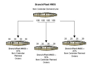

Setting Up Multifacility Planning

You set up multifacility planning to track supply, demand, and movement of material among the individual facilities of your enterprise. Multifacility planning provides a flexible method for planning supply and resupply activities.
In multifacility planning, you must set up a table of supply and demand relationships among your facilities. The system uses these relationships to generate and maintain multifacility plans.

Setting Up Supply and Demand Relationships

Use Branch Relationships Revisions (P3403T) to set up supply and demand relationships for any level of detail that you choose, including:

• Branch/plant
• Product group
• Master planning family
• Individual item number

This approach allows you to maintain supply and demand relationships in one central location, and reduce inventory errors caused by complex facility relationships. In addition, when you set up supply and demand relationships, you can use the following optional features:

Markup
You can have the system automatically mark up the cost of an item when you create a transfer order. The system can adjust the cost by a fixed amount or percentage.
Availability checking
You can ensure that the branch from which you are ordering has enough inventory in stock to fill the order. If the required quantity is not available, the system checks subsequent facilities in the sequence that you define.
Effectivity dates
Use effectivity dates to control the demands that are placed on your supply branches. If an effectivity date that was assigned to a supply branch has expired, the system checks for another facility.
The Material Requirements Planning (MRP), Distribution Requirements Planning (DRP), and Master Production Scheduling (MPS) versions of the Branch Relationships Revisions program use the same processing options. You can vary the settings in the processing options to accommodate the different requirements for a material requirements plan.
Caution
When you delete a supply and demand relationship, the system deletes the entire record.
To set up supply and demand relationships
From the Multi-Facility Setup menu (G3443), choose Branch Relationships Revisions.

1. On Work With Branch Relationships, complete one of the following fields:

• Supply Branch/Plant
• Demand Branch/Plant
• Use the View menu to switch from viewing the supply branch/plant to viewing the demand branch/plant. A processing option controls which branch/plant is the default.

2. To narrow your search, complete one of the following fields and click Find. Enter an item number to display all branch/plants that either supply or demand a certain part. Enter the planning family to display all branch/plants that either supply or demand parts that belong to a specific master planning family.

• Planning Family
• Item Number

3. Choose the record and click Select.
4. On Branch Relationship Revisions, complete the following fields:
Include/ Exclude
Some parts might come from certain branch/plants. In multifacility planning, if Exclude is selected, then the item is supplied by the demand branch only.
Effective From
This date defaults in from the bill of material.
Source Percent
The percent of demand to be supplied by the source branch/plant.
Percent To Fill
This amount of the source percent must be available to be filled by this branch/plant. The percent of demand should be filled to place a transfer order message. A transfer order is generated if Availability Check is on.
5. Complete the following optional fields, then click OK:
Branch Level
The branch that will go first, second, and so on. The lowest level is processed first (the highest numerical value). Ensure all demand is generated before supply is allocated.
Branch Priority
This field shows the sequence within a level branch/plant where requirements are processed.
Transfer Leadtime
This field shows the time to ship the item from the supply to the demand branch plant in days.
Availability Check
If availability check is on, the system checks the availability of the supply branch inventory only. The available balance is committed until a zero inventory balance, and then moves to another supply branch or creates an order in the demand branch.
If availability check is off, then the inventory balance can go negative.

Processing Options for Branch Relationships Revisions (P3403T)
Defaults
Enter the default Branch Relationship display mode.
1. 'D' = Demand branch 'S' = Supply branch
Enter a '1' to automatically update the Branch Level field.
2. Branch Level update

Note
You must set this processing option to ensure that the level of the component branch is one level higher than the header for the source branch. The branch level on the Defaults tab, along with the branch priority, determines the sequence in which the system processes supply and demand plants. The system processes the branches with the highest numerical branch levels first.
Reviewing Branch Relationships
Use the Branch Relationships Chart (P34031) to review supply and demand relationships in a graphical, hierarchical format. The Branch Relationships Chart displays the following:
Branch
Level of the branch
Supply branches for the corresponding demand branch
The Material Requirements Planning (MRP), Distribution Requirements Planning (DRP), and Master Production Scheduling (MPS) versions of the Branch Relationships Chart program use the same processing options. You can vary the settings in the processing options to accommodate the different requirements for a material requirements plan.
To review branch relationships
From Multi-Facility Setup (G3443), choose Branch Relationships Chart.
1. On Work With Branch Relationships Hierarchy, complete the following field to locate the branch/plant for which you want to display supply and demand relationships:
Supply Branch
2. To narrow your search to a specific level of detail, complete one of the following optional fields and then click Find:
Item Number
Plan Family
3. On Work With Branch Relationships Hierarchy, choose a row and click Select to review the branch relationships.


Transfer Orders and Multifacility Planning
Transfer orders are used by the Multifacility Planning system to transfer inventory between branch/plants within your company. The transfer of inventory is done by generating a purchase order at the demand plant and a sales order at the supply plant.
Instead of manually entering the transfer orders, you run Master Planning Schedule – Multiple Plant (R3483), which generates the plan and respective planning messages. You then process the messages.
When the system creates a transfer order from a planning message, the system does the following:
Creates a purchase order for the supply branch/plant that ships the items
Creates a sales order for the demand branch/plant that receives the items
Processes the inventory amounts on the transfer order as a formal purchase and sale of goods
Creates documents—such as orders, pick slips and invoices—that are necessary to complete the transfer
When the sales order is generated, the system uses the Customer Master for certain defaults and validation. The system might check the following settings:
availability checking
partial shipments allowed
default carrier
order holds
freight charges
Markups can also be applied by setting up the Branch Relationships Master File table (F3403).
When the purchase order is generated, the system uses the supplier master to get defaults and validation. The system might check the following settings:
order holds
print messages
landed costs
JD Edwards EnterpriseOne software has standard document types set up for transfer orders. Sales orders use document type ST and purchase orders use OT. These document types are defined in user defined code (UDC) table 00/DT. Thus, you can create your own document types. For example, transfers that are generated by planning might use the ST/OT document types; orders generated manually use alternate document types. Along with the visible difference in document type, the use of different document types allows for differences in accounting, approvals, and order activity rules.
Customer and Supplier Masters and Multifacility Planning

To create transfer orders in the Multifacility Planning system, you are required to set up default customer and supplier masters for the branch/plants that are used.

Note
Transfer orders use the customer and supplier masters in unique ways during order generation.
A customer master is required for the demand plant, and a supplier master is required for the supply plant.
A standard sales order uses the customer address book number for the billing instructions. The sales order that is created for a transfer order uses the address number of the branch from which you are shipping.
A standard purchase order uses the supplier’s address book number. The purchase order that is created for a transfer order uses the address book number of the branch that is receiving the product.
Generating Multifacility Plans
Use one of the following navigations:
From the Multi-Facility Planning menu (G3423), choose MPS Regeneration.
From the Multi-Facility Planning menu (G3423), choose MRP Regeneration.
After you have set up the supply and demand relationships among your branch/plants, you can use the Distribution Requirements Planning (DRP), Master Production Scheduling (MPS), and Material Requirements Planning (MRP) gross regeneration versions of Master Planning Schedule – Multiple Plant (R3483) to generate a multifacility plan. Alternatively, you can use the DRP, MPS, and MRP net change versions of Master Planning Schedule – Multiple Plant to generate a multifacility plan.
When you generate a multifacility plan, the system evaluates selected information, performs calculations, and recommends a time-phased plan for all selected items.
Prerequisite
q Set up DRP/MPS multifacility planning.

Processing Options for Master Planning Schedule – Multiple Plant (R3483)
Horizon Tab
These processing options specify dates and time periods that the program uses when it creates the plan.
1. Generation Start Date
Use this processing option to specify the date for starting the planning process. This date is also the beginning of the planning horizon.
2. Past Due Periods
3. Planning Horizon Periods
Number of planning days
Use this processing option to specify the number of days from the horizon start date for which you want to see daily planning data.
Number of planning weeks
Use this processing option to specify the number of weeks for which you want to see weekly planning data, following the daily data.
Number of planning months
Use this processing option to specify the number of months for which you want to see monthly planning data, following the weekly data.
Parameters Tab
Use these processing options to define processing criteria. The following information concerns your choice of generation type:
Generation Type 1, single-level MPS/DRP. You can use this generation type either in a distribution environment for purchased parts with no parent-to-component relationship, or in a manufacturing environment with parent-to-component relationships. When you use this generation type, the system performs the following actions:
Produces a time series for each item that you specify in the data selection with a Planning Code of 1 on the Plant Manufacturing Data tab of the Work with Item Branch form. This code indicates whether the item is manufactured or purchased.
Does not explode demand down to the components for manufactured items. Use generation type 1 if you first want to process only the master-scheduled end-items. Thus, you can stabilize the schedule before placing demand on the components.
Does not create pegging records.
Generation Type 3, multilevel MPS. This generation type is an alternative to generation type 1 and performs a complete top-to-bottom processing of master-scheduled items. For all parent items that you specify in the data selection, the program explodes demand down to the components. You must specify all of the items to be processed in the data selection, not just the parent items. The program also creates pegging records.
Generation Type 4, MRP with or without MPS. This generation type performs the same functions as generation type 3. After you perform a complete generation and stabilize your master schedule, you can limit data selection to MRP items (with planning codes of 2 or 3), thereby reducing processing time. This action is possible because the system still stores demand from the master-scheduled items in the MPS/MRP/DRP Lower Level Requirements File table (F3412).
Generation Type 5, MRP with frozen MPS. This generation type freezes the master schedule after it has been stabilized. Before using this generation type, make all necessary adjustments to master-scheduled items and release orders to provide supply for the demand. This generation type freezes the entire planning horizon, which is similar to the way the freeze fence freezes a part of the horizon. Running this generation type produces the following results, which apply to MPS items only:
No new orders will be planned.
No messages for existing orders will be created.
The adjusted ending available quantity can be negative.
Demand is only exploded down to components from existing work orders. No -PWO demand from parent items exists; only -FWO demand exists.
1. Generation Mode
1 = net change
2 = gross regeneration
A gross regeneration includes every item specified in the data selection. A net change includes only those items in the data selection that have changed since the last time you ran the program.
Valid values are:
1 net change
2 gross regeneration
2. Generation Type
1 = single level MPS/DRP
3 = multi-level MPS
4 = MRP with or without MPS
5 = MRP with frozen MPS
Please see the help for the Parameters tab for detailed information.
Valid values are:
1 single-level MPS/DRP
3 multi-level MPS
4 MRP with or without MPS
5 MRP with frozen MPS
3. UDC Type
Use this processing option to specify the UDC table (system 34) that contains the list of quantity types to be calculated and written to the Time Series table (F3413). Default = QT.
4. Version of Supply/Demand Inclusion Rules

Use this processing option to define which version of supply/demand inclusion rules the program reads. These rules define the criteria used to select orders for processing.

On-Hand Tab
These processing options define how the program calculates on-hand inventory.
1. Include Lot Expiration Dates
blank = do not include
1 = include
Use this processing option to specify whether the system considers lot expiration dates when calculating on-hand inventory. For example, if you have 200 on-hand with an expiration date of August 31, 2005, and you need 200 on September 1, 2005, the program does not recognize the expired lot and creates a message to order or manufacture more of the item to satisfy demand.
Valid values are:
blank do not consider lot expiration dates when calculating on-hand inventory
1 consider lot expiration dates when calculating on-hand inventory
2. Safety Stock Decrease
blank = do not decrease
1 = decrease
Use this processing option to specify whether to plan based on a beginning available quantity from which the safety stock quantity has been subtracted.
Valid values are:
blank do not decrease
1 decrease
3. Receipt Routing Quantities
Quantity in Transit
blank = do not include in on-hand inventory
1 = include in on-hand inventory
In a manufacturing environment, sometimes it is necessary to establish where stock is, in order to determine whether or not it is available for immediate use. Enter 1 if you want quantities in transit to be included in the Beginning Available calculation on the time series. Otherwise, the program includes these quantities in the In Receipt (+IR) line of the time series. The quantities are still considered available by this program. The difference is only in how you view the quantities in the time series.
Valid values are:
blank do not include in on-hand inventory
1 include in on-hand inventory
Quantity in Inspection
blank = do not include in on-hand inventory
1 = include in on-hand inventory
Use this processing option to specify whether to include quantities in inspection when the system calculates the Beginning Available amount. Otherwise, the system includes these quantities in the In Receipt (+IR) line of the time series. The system still considers the quantities available, but the way in which you view the quantities in the time series differs. Valid values are:
Blank
Do not include quantities in on-hand inventory
1
Include quantities in on-hand inventory
User Defined Quantity 1
blank = do not include in on-hand inventory
1 = include in on-hand inventory

In a manufacturing environment, sometimes it is necessary to establish where stock is, in order to determine whether or not it is available for immediate use. Enter 1 if you want these user defined quantities (defined on Receipt Routings Revisions in the Update Operation 1 field) to be included in the Beginning Available calculation. Otherwise, the program includes these quantities in the In Receipt (+IR) line of the time series. The quantities are still considered available by this program. The difference is only in how you view the quantities in the time series.
Valid values are:
blank do not include in on-hand inventory
1 include in on-hand inventory
User Defined Quantity 2
blank = do not include in on-hand inventory
1 = include in on-hand inventory
In a manufacturing environment, sometimes it is necessary to establish where stock is, in order to determine whether or not it is available for immediate use. Enter 1 if you want these user defined quantities (defined on Receipt Routings Revisions in the Update Operation 2 field) to be included in the Beginning Available calculation. Otherwise, the program includes these quantities in the In Receipt (+IR) line of the time series. The quantities are still considered available by this program. The difference is only in how you view the quantities in the time series.
Valid values are:
blank do not include in on-hand inventory
1 include in on-hand inventory
4. Lot Hold Codes ( up to 5 )
blank = include no held lots in calculation of on-hand inventory
* = include all held lots in calculation of on-hand inventory
Use this processing option to specify the lots to be included in the calculation of on-hand inventory. You can enter a maximum of 5 lot hold codes (41/L). blank include no held lots in calculation of on-hand inventory * include all held lots in calculation of on-hand inventory
5. Include Past Due Rates as a supply
blank = do not include
1 = include
Use this processing option to specify whether the system considers open quantity from past due rate orders as supply. If you enter 1, open quantities from past due rate orders are included in the rate schedule unadjusted (+RSU) line as well as the rate schedule adjusted (+RS) line of the Master Planning Schedule - Multiple Plant program (R3483). Valid values are:
Blank
Do not consider past due orders as supply.
1
Consider past due orders as supply.
Forecasting Tab
These processing options serve the following two purposes:
They determine which forecast types the program reads as demand
They initiate special logic for forecast consumption
1. Forecast Types Used ( up to 5 )
Forecasts are a source of demand. You can create forecasts using 12 different forecast types (34/DF) within the Forecasting system. One is considered the Best Fit (BF) type compared to an item's history of demand. Use this processing option to define which forecast quantities created by which forecast type are included in the planning process. Enter multiple values with no spaces, for example: 0102BF.
2. Forecast Consumption Logic
blank = do not use forecast consumption
1 = use forecast consumption
2 = use forecast consumption by customer
Use this processing option to specify whether the system uses forecast consumption. If you use forecast consumption, any sales order due in the same period as the forecast is included as part of the forecast for that period. The sales order is not considered an additional source of demand. For forecast consumption to be used, the planning fence rule for the item must be H and the planning fence must be 999. You enter these values on the Plant Manufacturing Data form.
Note: When you use forecast consumption, the system applies forecast consumption logic to the aggregate sales order and forecast quantities.
Blank
Do not use forecast consumption.
1
Use forecast consumption.
3. Interplant Demand Consumes Forecast
blank = do not use
1 = use
When using forecast consumption, use this processing option to specify whether to use interplant demand to consume forecast. When using any other planning rule, you can use this option to specify whether to consider interplant demand as customer demand. When the option is set, the system considers interplant demand for firm and planned transfer orders.
When the option is blank, the system ignores interplant demand by forecast consumption or planning rules and considers interplant demand as a separate source of demand. Valid values are:
Blank Do not consider interplant demand as customer demand.
1 Consider interplant demand as customer demand.


Document Types Tab
These processing options establish default document types.
1. Purchase Orders
When you receive messages related to purchase order creation, this document type will appear as the default. The default value is OP.
2. Work Orders
When you receive messages related to work order creation, this document type will appear as the default. The default value is WO.
3. Rate Schedules
When you receive messages related to rate schedule creation, this document type will appear as the default. The default value is AC.


Leadtimes Tab
These processing options let you specify safety leadtimes to allow extra time for delays in receipt or production. Use damper days to filter out unwanted messages.
1. Purchased Item Safety Leadtime
For items with stocking type P, the program adds the value you enter here to the item's level leadtime to calculate the total leadtime.
2. Manufactured Item Safety Leadtime
For items with stocking type M, the program adds the value you enter here to the item's level leadtime to calculate the total leadtime.
3. Expedite Damper Days
Use this processing option to specify the number of days before the system generates an expedite message. If the number of days between the date when the order is actually needed and the due date of the order is less than the number of days entered here, the system does not generate an expedite message.
4. Defer Damper Days
Use this processing option to specify the number of days before the system generates a defer message. If the number of days between the date when the order is actually needed and the due date of the order is less than the number of days entered here, the system does not generate a defer message.
Performance Tab
These processing options define output and specify conditions that might decrease processing time.
1. Clear F3411/F3412/F3413 Tables
blank = do not clear tables
1 = clear tables
Use this processing option with extreme caution! If you enter 1, all records in the MPS/MRP/DRP Message table (F3411), MPS/MRP/DRP Lower Level Requirements (Pegging) table (F3412), and MPS/MRP/DRP Summary (Time Series) (F3413) table are purged.
Access to this program should be limited. If multiple users run this program concurrently with this processing option set to 1, a record lock error results and prevents complete processing.
Valid values are:
blank do not clear tables
1 clear tables
2. Initialize MPS/MRP Print Code
blank = do not initialize the Item Branch file
1 = initialize the Item Branch file
If you enter 1 in this processing option, the program initializes every record in the Item Branch table (F4102) by setting the Item Display Code (MRPD) to blank
If you leave this field blank, processing time is decreased. The system will not clear the records in the Item Branch table (F4102).
Regardless of how you set this processing option, for each item in the data selection the MRPD field is updated as follow:
o 1 if messages were not created
o 2 if messages were created
The Print Master Production Schedule program (R3450) allows you to enter data selection based on the MRPD field.
Valid values are:
blank Do not initialize the Item Branch file.
1 Initialize the Item Branch file.
3. Messages And Time Series For Phantom Items
blank = do not generate
1 = generate
Use this processing option to specify whether the program generates messages and time series for phantom items.
Valid values are:
blank do not generate
1 generate
4. Ending Work Order Status
blank = all messages exploded
Use this processing option to specify the work order status at which messages are no longer exploded to components. If you leave this field blank, all messages are exploded to components.
5. Extend Rate Based Adjustments
blank = do not extend
1 = extend
Use this processing option to specify whether adjustments for rate based items are exploded to components, thereby creating messages for the components.
Valid values are:
blank do not extend
1 extend
6. Closed Rate Status
Use this processing option to specify the status of closed rates. When you plan for a rate-based item, the system does not process rate orders that are at a closed-rate status or a higher status.
Mfg Mode Tab
These processing options specify integration with other systems.
1. Process Planning
blank = discrete
1 = process
If you use process manufacturing, enter 1 to generate the plan based on the forecasts of the co-/by-products for the process. The program then creates messages for the process.
Valid values are:
blank discrete
1 process


Multi-Facility Tab
These processing options define criteria for a multifacility environment.
1. Date Branch
Enter the default branch/plant from which to retrieve the shop floor calendar.
If you leave this field blank, the calendar for each branch/plant is used and processing time increases.
2. Consolidation Method
1 = simple consolidation
2 = branch relationships ( default )
The simple consolidation method (1) adds the supply and demand for each branch, calculates a new time series, and places the result in the consolidated branch specified in the Consolidation Branch processing option.
The branch relationships method (2) uses the Branch Relationships table. This is the default.
Valid values are:
1 simple consolidation
2 branch relationships (default)
3. Consolidation Branch
If your consolidation method is 1 (simple consolidation), enter the branch/plant to contain the consolidated results. If the consolidated branch/plant also contains its own time series data, that data is included in the totals.
4. Category Code
1 = 41/P1
2 = 41/P2
3 = 41/P3
4 = 41/P4
5 = 41/P5
If your consolidation method is 2 (branch relationships), enter the category code of the part that is supplied by one branch/plant to another. There are five user defined category code tables.
Valid values are:
1 41/P1
2 41/P2
3 41/P3
4 41/P4
5 41/P5
5. Manufacture At Origin
blank = create transfer orders for manufactured and purchased items
1 = create transfer orders only for purchased items
Enter 1 if there are manufactured and purchased items in the same category code, but you only want to obtain the purchased items from another branch/plant. Transfer order messages are created for purchased items, and work order messages are created for manufactured items.
Valid values are:
blank create transfer orders for manufactured and purchased items
1 create transfer orders only for purchased items
6. Transfer Order Document Type
blank = OT
When you receive messages related to transfer order creation, this document type will appear as the default. The default value is OT.


Parallel Tab
These processing options specify the number of processors that the system uses during parallel processing. These processing options also specify whether the system runs preprocessing during parallel processing.
1. Number of Subsystem Jobs
0 = Default
Use this processing option to specify the number of subsystems in a server.
The default is 0 (zero).
2. Pre Processing
blank = Do not perform pre processing
1 = Perform pre processing
Use this processing option to specify whether the system runs preprocessing during parallel processing. During preprocessing, the system checks supply and demand and plans only the items within supply and demand. Preprocessing improves performance when you run MRP and is valid only when the number of items actually planned is less than the total number of items in the data selection. Valid values are:
Blank The system does not run preprocessing.
1 The system runs preprocessing.
Working with Multifacility Planning Output

Multifacility planning output consists of information in the time series and transfer order messages. Use the time series information to either accept or override the planning that the system suggests. You should review the transfer order messages for individual item numbers to determine which action, if any, that you need to take.
Reviewing the Time Series for the Multifacility Schedule
To review the multifacility time series
From the Multi-Facility Planning Daily Operations menu (G3414), choose Time Series/ATP Inquiry.
1. On Work With Time Series, complete the following fields and click Find to locate the time series for an item:
Item Number
Branch/Plant
Processing Transfer Order Messages for the Multifacility Schedule
Use MRP/MPS Detail Message Revisions (P3411) to review the transfer order messages for the multifacility schedule. Multifacility scheduling creates messages that are appropriate to the demand and supply facilities. If you process the messages, the system automatically creates transfer orders. You can transfer items between facilities either at cost or at a markup.
To process multifacility transfer order messages
From the Multi-Facility Planning Daily Operations menu (G3414), choose Detail Message Review.
1. On Work With Detail Messages, complete the following fields and click Find to locate the transfer order messages for an item:
Item Number
Demand Branch
2. Choose the transfer order messages that you want to process.
3. From the Row menu, choose Process Message(s) to create the following:
Transfer order for the item
Purchase order number for the demand plant
Sales order number for the supply plant
4. On Work With Detail Messages, review the information for the new orders in the following fields:
Order Number
Start Date
Request Date
Recmd'd Start Date
Recmd'd Complete
Demand Branch
Supply Branch
Multifacility Forecast Consumption
Multifacility forecast consumption in Material Requirements Planning (MRP) is a process to reduce the forecast quantity through the number of sales orders and shipped orders. The goal of forecast consumption is to have your forecast quantity be greater than the total of sales orders and shipped orders. The forecast quantity is consumed either fully or partially. For example, when the sales order quantity is greater than the forecast quantity, then the forecast quantity is fully consumed. The option that you choose is dependent on your need to forecast interplant demand.
Time Series Quantity Types
The system uses the following quantity types (34/QT) for multifacility consumption:
Calculations
If the Interplant Demand processing option for the Master Planning Schedule - Multiple Plant program (R3483) is on, the transfer orders consume the supply plant's forecast. The system does not plan the transfer orders again. The system uses the following calculations when the Interplant Demand processing option is on:
-TIU = (-SOU) + (-ID) + (-FID)
+PLO = (-FSCT) + (-TI)
If the Interplant Demand processing option is off, the system processes the transfer orders as additional demand for the supply plant. The system uses the following calculations when the Interplant Demand processing option is off:
(TIU) = (-SOU)
+PLO = (-FSCT) + (-FID) + (-TI) + (-ID)
Additional Options for Multifacility Forecast Consumption
To have interplant demand consume forecast, you need to add your transfer order type to user defined code (UDC) table 40/CF. The system then accumulates ship-confirmed transfer orders to accumulate in the -SHIP quantity type while still using the orders to consume forecast. Also, regardless of the Interplant Demand processing option, the system processes interplant demand consistently whether the order is planned demand or firm demand. For example, interplant demand either consumes or does not consume forecast.
If you do not want to use the new quantity types, you can make a copy of the 34/QT table with the necessary quantity types. The system completes the calculations but does not display them on the time series. The system displays the following results when you remove the following quantity types:

Introduction to Standard Costing

Standard costing is an important subtopic of manufacturing cost accounting. Standard costs are associated with manufacturing companies and are utilized to manage the costs of direct material, direct labor, and manufacturing overhead.

In lieu of assigning actual or average costs of direct material, direct labor, and manufacturing overhead and rolling these costs into their products, most manufacturers assign a standard cost to their systems. This means that their inventories and cost of goods sold are valued using the standard costs, and not the actual or average costs, of a product. The Manufacturers pays their vendors at actual costs which can vary over time. This results in differences between the actual costs and the standard costs, and those differences are known as variances.

Standard costing and the related variances are valuable to measure the performance of inventory and product production. When a variance arises, management becomes aware that manufacturing costs have differed from the standard (planned, expected) costs.

• If the actual cost is greater than the standard cost the variance is referred to as unfavorable; and unfavorable variances result in the company’s actual profit being less than planned.
• If the actual cost is less than the standard cost the variance is referred to as favorable; and favorable variances result in the company’s actual profit being less planned.
  Timely reporting of these manufacturing variances allows management to take action on the differences from the planned amounts.

This, however, is not the only reason that manufacturers utilize standard costs. In the manufacturing process, materials are issued to work orders and job orders and taken out of the perpetual inventory and show up on the balance sheet on what is known as work in process. Because work in process no longer has any part number identity, it is retained as a gross value on the balance sheet. If a part is issued to a work order and the value of that part is written to the general ledger work in process account at its current value. If the company were using average cost to value their products and the item in question is received at a higher price prior to the work order being completed, then the item will be relieved from inventory in the future at the new value, causing a negative balance in the work in process account. Multiply this by thousands of transactions and you will see why it is important to utilize standard costs in a manufacturing system.

The perpetual inventory is maintained at standard cost (including Direct Materials and Subassemblies), and the standard cost of finished goods becomes the sum of the standard costs of the following values:

• Direct material
• Direct labor
• Manufacturing overhead
• Variable manufacturing overhead
• Fixed manufacturing overhead

Increased Business Value With Collaborative Manufacturing

In today’s emerging global economy, seamless communication does not stop at the four walls of the plant. Sharing information in real time both within the enterprise and beyond is an essential component to maintaining information integrity and achieving operational excellence. This communication must also include supply chain-wide notification of status and events in real time to effectively link a global network of suppliers, manufacturers and customers. The right manufacturing execution solution will empower manufacturers to achieve seamless integration across their business systems and software—while protecting IT investments and customer relationships. It will achieve this by integrating Web-based solutions directly with enterprise and business-to-business applications. A manufacturing execution solution should also provide the platform for real-time information flow, eliminate process gaps and deliver competitive advantage—eliminating the delays and errors caused by systems which cannot effectively share operational data.

Finding the Right Manufacturing Execution Solution for Your Unique Environment
As you move toward coupling your manufacturing operations tightly with logistics, transportation and customer demand, finding the right solution is key. As with any enterprise-wide software evaluation process, there are a handful of important questions that must be answered prior to selecting a vendor. You must be able to find a solution that addresses your business’ specific pain points at a cost that works within your budget. For each vendor involved in the selection process, it is essential that your selection team gather detailed responses to the following issues:

• Breadth of technology - Does the vendor offer a wide range of supply chain-related solutions that integrate easily on the same platform? Does it have experience integrating with a variety of software and hardware systems? Does it have a history of releasing product upgrades containing new functionality that demonstrates a commitment to excellence in the space?


• Ability to adapt to change - How does the vendor approach changes to your system as your requirements shift? Does it utilize costly custom code? Do these changes carry forward during an upgrade?


• Company history - Has the company been in business for a number of years? Does it have a track record of solving problems for manufacturers? Does the product line demonstrate progressively more complex technologies developed using the most advanced toolsets?


• Financial stability - Will the company be around in three years to support the system you have purchased? Are the vendor’s sales growing? Does the company have a sufficient amount of emergency capital in case of an economic downturn?


• Customer base - Does the vendor have a long list of satisfied customers? Are the majority of these customers referenceable? Can the vendor prove it can keep customers happy over the long term?


• Implementation success - Has the company ever had a failed implementation? If so, how recently? What were the reasons?

Leveraged ERP Investment

Manufacturers that have implemented an ERP system have invested significant effort (and money) creating an enterprise software solution. Despite these investments, manufacturers often find their ERP systems do not provide the results they expected on the shop floor. ERPs often fall short because they are overly complex, difficult for shop floor employees to use, and rooted in traditional MRP batch-based processing. A manufacturing execution solution is designed to leverage an ERP investment, not replace it.
Manufacturing execution solutions address these issues by providing intuitive execution capabilities based on a real-time, lean execution philosophy. This means manufacturers get the best of both worlds—easy-to-use execution tools for the shop floor that also support planning decisions by continuously feeding real-time transaction information to the ERP. Manufacturing execution solutions share information with the ERP in real time, allowing the ERP to have an accurate representation of shop floor activities. With real-time visibility to execution, the ERP makes intelligent decisions about supply/demand matching and order promising.

Reduced Cost of Regulatory Compliance
Manufacturing environments are becoming increasing regulated. Whether the compliance requirement is for the FDA or Sarbanes-Oxley, the costs associated with achieving compliant processes can be excessive. With a rich transaction history that provides detailed audit trails and electronic approval processes, a manufacturing execution solution will facilitate compliant processes without excessive paperwork and manual work-arounds. Additionally, a manufacturing execution solution is designed to be responsive to change over time. This means that new regulatory requirements are easily met without system upgrades or customizations.

Personalized Manufacturing
Customer-specific manufacturing is a trend driving increased complexity and cost for today’s manufacturers. Customer specific bills of materials, routings and test instructions are challenging to manage, but can be a source of competitive differentiation. Manufacturing execution solutions respond to this challenge by offering personalization capabilities that meet today’s customer requirements and adapt to meet tomorrow’s unforeseen demands.
The ability to personalize a manufacturing execution solution is a key benefit—but not one that all applications offer. The greatest level of benefit will be achieved through a solution that accommodates personalization via configuration tool sets. With this type of platform, configurations can be made easily and cost-effectively. This means the manufacturers—not the solution vendors—truly own the system. With a flexible manufacturing execution solution, there is no custom coding required for configuration; changes carry over and workflow can be altered as needed after the system go-live. The result of this is that the system’s total cost of ownership is greatly reduced over the lifetime of the application.

Focused Technology Approach
With the most robust manufacturing execution solutions, nearly any station or work cell in the facility can be integrated into the system and either monitored, controlled or reported against. Machines, scales, gauges, statistical process control (SPC) systems, PLCs, label printers, serial devices, PDAs, automated material handling equipment, wired and wireless terminals, and RFID systems are integral parts of manufacturing execution—and the best manufacturing execution solutions will integrate seamlessly with all of them. Manufacturing execution solutions often feed multiple host systems and facilitate reporting beyond the current capabilities of many ERP systems.
Solving the problems inherent in today’s manufacturing environment is best accomplished using a modular technology approach. Manufacturing execution solutions start with bar code or RFID data acquisition to improve order visibility and extend beyond basic data collection as appropriate in each company’s individual situation. This allows for a right-sized application based on current business needs and areas requiring the most attention. Oftentimes, this provides self funding for future projects because ROI is generated quickly.

Continuous Improvement: “Adapt or Fail”

Manufacturers have learned that staying competitive means they must continually improve their processes or face the consequences of technological Darwinism—”adapt or fail.” Whether the initiative is Six Sigma or kaizen, traditional implementations of JDEdwards EnterpriseOne are nearly impossible to change when needed because they require expensive, time consuming custom code-based modifications. Because of this, the software becomes a barrier to operational excellence. This usually means that improvement opportunities are lost, or work-arounds are developed to accomplish tasks outside of the system. This results in poor data accuracy.
A new approach, called Lean Execution™ has recently been compiled on the belief that software should be a catalyst for continuous improvement—not an obstacle. Our implementation methodology not only provides a detailed view of plant history, but the flexible architecture also allows reconfiguration quickly and cost-effectively as the manufacturing operations change and evolve. We also provide the Business Intelligence needed to make fact-based decisions and adapt as manufacturing operations improve over time.
Maximized Supplier Relationships
In today’s lean and just-in-time manufacturing environments, collaboration with key suppliers is essential. The best manufacturing execution solutions provide manufacturers with the capability to exchange information among trading partners and enable true collaborative execution up and down the supply chain. A secure Web portal replaces time consuming phone calls and faxes as the basis for real-time information sharing and improved inventory visibility—critical factors in enhancing collaboration and streamlining supply chain operations.
Some manufacturing execution solutions also provide both the communication and visibility necessary to facilitate the effective delivery of goods from supplier to buyer. From the point of purchase order (PO) release at the buyer’s location through fulfillment, shipment and receipt, processes that have historically been performed manually—or in some cases simply not performed—are automated. With improved communication regarding compliance and/or serialized labeling requirements, inventory is received at the dock door with the required bar codes already applied. Functionality can also be provided to allow suppliers to perform other value-added services for their customers, including demand-pull replenishment, advanced shipping notification (ASN), and supplier quality inspections.
Rapid Product Recall Decisions
Product safety and quality are paramount concerns for manufacturers. When there are concerns about safety or quality, it is essential for manufacturers to have traceability tools that assist them in making product recall decisions. Manufacturing execution solutions aid in this process by capturing detailed product genealogies. When suppliers communicate a product defect, it is possible to trace exactly which finished goods were manufactured using the supplier’s defective component. This traceability can be achieved using lot number, serial number or other product attribute such as version, revision or “born-on date.”
Product recalls often result in enormous costs for the company issuing the recall. In most cases, companies lack information about the affected products. This results in companies inspecting individual products, or being overly cautious and recalling products that have no risk of quality or safety issues. Manufacturing execution solutions bridge this information gap for many manufacturers. With detailed product and order history information, these systems help companies deal with recalls in a timely, cost-effective manor.

Strengthened Decision-Making Based on Real-Time Information

A Lean Execution™ implementation supplies key personnel the decision-making data necessary to optimize manufacturing performance. From any location, the technology will allow managers to make immediate decisions on staffing, maximize labor efficiencies, control order fulfillment and monitor machine utilization. Real-time performance reports such as actual versus plan, production unit cycle time, production efficiency, scrap and downtime by machine or work cell can all be specifically configured for up-to-the-second review and action by management.
When unexpected events do occur, Lean Execution™ also helps managers and lead operators take proactive steps by utilizing your customized set of alerts and alarms. Using workflow notification key individuals are notified about potential issues—before they become costly problems. Manufacturing execution solutions do not stop after notifying operators of unexpected events. This type of system pairs event notification with appropriate workflow so operators take suitable resolution steps in real time without affecting operations.

Production order status and work in process are readily accessible via standard JDE Video Screens. This can also empower managers and other decision-makers to communicate information electronically to customers and other manufacturing locations. Ease of information access also smoothes the daily transition between shift managers and provides updated statistics on key performance indicators (KPI), wellness views and other important reports.

Lean Execution™ With JDEdwards EnterpriseOne

Fast Cost Reduction
Now that we have defined how proper implementation of JDE Manufacturing can create “paperless shop floor environments,” the next question to be answered is “What benefits will my company realize?”

Increased Levels of On-Time and Complete Shipments
JDEdwards provides the workflow, visibility and event notification required to ensure that manufacturing is meeting customer demand. Additionally, these systems reduce non value-added activity, increase data accuracy and provide the other ERP systems with the real-time data needed to maximize processing, planning and scheduling activities. This results in the ability to increase levels of on-time and complete shipments.
As stated earlier Lean Execution™ requires putting information in the hands of those who actually handle the inventory or produce the products. This is sometimes the biggest stumbling block in entire process because managers and supervisors don’t readily believe that the production and manufacturing workers can be trained to input the correct data. However, once this hurdle is overcome the solution creates a paperless environment by giving operators instant access to work instructions and CAD drawings, so they always have the up to date information required to build products that meet the customers’ demanding specifications.
More importantly, having information about events as they occur allows decision makers to easily identify or prevent potential problems and bottlenecks. For example, the planners may already be well aware of the problems created by shortages of key manufacturing materials that may halt production, shipments arriving late or incomplete, and backorders; however, with a few properly implemented steps the material pickers, the purchasing agent and the receiving department can also be updated as to the status of critical parts. Additionally, the lack of visibility into machines operating outside control limits or processes not meeting appropriate yields can ultimately delay customer shipments. With JDE Workflow, real-time notification of events and exceptions—often before they occur—allows the appropriate parties to take proactive steps to manage them. This will likely save the cost of expediting shipments that were unexpectedly completed late. Ultimately, the ability to keep costs in check, production and shipments on schedule, and customers happy increases bottom line profitability.
By streamlining data acquisition and execution for operators on the factory floor, it is possible to create efficient processes that consist only of the value-added activities. The result is a lean and efficient environment. Additional investment can be made into mobile data terminals for material handlers or strategically placed WIP stations or terminals on the factory floor, workers can then be directed to perform tasks and collect information in real time using either third party tools or standard user interfaces. In addition, new employee training time is significantly reduced, while workflow notification and electronic communication provides cross training opportunities within the existing workforce. Lean Execution™ solutions empower JDEdwards EnterpriseOne users to easily implement and manage truly paperless manufacturing processes.

JDE Setting Up Supply and Demand Relationships

Use Branch Relationships Revisions (P3403T) to set up supply and demand relationships for any level of detail that you choose, including:
· Branch/plant
· Product group
· Master planning family
· Individual item number
This approach allows you to maintain supply and demand relationships in one central location, and reduce inventory errors caused by complex facility relationships. In addition, when you set up supply and demand relationships, you can use the following optional features:
Markup
You can have the system automatically mark up the cost of an item when you create a transfer order. The system can adjust the cost by a fixed amount or percentage.
Availability checking
You can ensure that the branch from which you are ordering has enough inventory in stock to fill the order. If the required quantity is not available, the system checks subsequent facilities in the sequence that you define.
Effectivity dates
Use effectivity dates to control the demands that are placed on your supply branches. If an effectivity date that was assigned to a supply branch has expired, the system checks for another facility.
The Material Requirements Planning (MRP), Distribution Requirements Planning (DRP), and Master Production Scheduling (MPS) versions of the Branch Relationships Revisions program use the same processing options. You can vary the settings in the processing options to accommodate the different requirements for a material requirements plan.
Caution
When you delete a supply and demand relationship, the system deletes the entire record.
To set up supply and demand relationships
From the Multi-Facility Setup menu (G3443), choose Branch Relationships Revisions.
1. On Work With Branch Relationships, complete one of the following fields:
· Supply Branch/Plant
· Demand Branch/Plant
Use the View menu to switch from viewing the supply branch/plant to viewing the demand branch/plant. A processing option controls which branch/plant is the default.
2. To narrow your search, complete one of the following fields and click Find. Enter an item number to display all branch/plants that either supply or demand a certain part. Enter the planning family to display all branch/plants that either supply or demand parts that belong to a specific master planning family.
· Planning Family
· Item Number
3. Choose the record and click Select.
4. On Branch Relationship Revisions, complete the following fields:
· Include/ Exclude
Some parts might come from certain branch/plants. In multifacility planning, if Exclude is selected, then the item is supplied by the demand branch only.
· Effective From
This date defaults in from the bill of material.
· Source Percent
The percent of demand to be supplied by the source branch/plant.
· Percent To Fill
This amount of the source percent must be available to be filled by this branch/plant. The percent of demand should be filled to place a transfer order message. A transfer order is generated if Availability Check is on.
5. Complete the following optional fields, then click OK:
· Branch Level
The branch that will go first, second, and so on. The lowest level is processed first (the highest numerical value). Ensure all demand is generated before supply is allocated.
· Branch Priority
This field shows the sequence within a level branch/plant where requirements are processed.
· Transfer Leadtime
This field shows the time to ship the item from the supply to the demand branch plant in days.
· Availability Check
If availability check is on, the system checks the availability of the supply branch inventory only. The available balance is committed until a zero inventory balance, and then moves to another supply branch or creates an order in the demand branch.
If availability check is off, then the inventory balance can go negative.
Processing Options for Branch Relationships Revisions (P3403T)
Defaults
Enter the default Branch Relationship display mode.
1. 'D' = Demand branch 'S' = Supply branch
Enter a '1' to automatically update the Branch Level field.
2. Branch Level update

Note
You must set this processing option to ensure that the level of the Demand Branch is one level higher than the header for the Supply branch. The branch level on the Defaults tab, along with the branch priority, determines the sequence in which the system processes supply and demand plants. The system processes the branches with the highest numerical branch levels first.

History of Computer Planning Systems

MRP I (1970’s) Materials Requirements Planning
MRP II (1980’s) Manufacturing Resources Planning
DRP (Late 1980’s) Distribution Resources Planning
ERP (1990’s) Enterprise Resources Planning
MRP
Inventory Data – time phased net requirements
Master Production Schedule – used actual demand
BOM – exploded to lower level requirements.

MRP – a set of techniques which used BOM’s, inventory data and the MPS to calculate requirements for materials.
• Makes recommendations to release replenishment orders for material.
• Makes recommendations to reschedule open orders when due dates and need dates are not in phase.
Provided a short–range plan to cover material requirements that were needed to make a product. Material Planning Operations analyzed demand from all operations, including:
Central and satellite distribution centers and warehouses rate–based repetitive manufactured items, process and discrete manufactured items engineer–to–order contracted items, maintenance/ repair, operational items for plant and equipment maintenance, supplier–managed inventory.

Master Production Scheduling (MPS)

A schedule of items and quantities that a company expects to manufacture. In MRP it used actual demand.

Material Planning (MRP)

Used the master production schedule, the bill of materials, and inventory records to calculate time–phased net requirements for every item, and created a plan for covering material requirements.
MRP II
Forecasting
Comprehensive formulae to plan the future
Resources Planning (CRP)
Labor and machine capacity analysis
Manufacturing Cost Accounting
Integrate costing and manufacturing
Production Activity Control
Feedback mechanisms

MRP II is a method for the effective planning of all resource of a manufacturing company. Ideally, it addresses operational planning in units, financial planning in dollars, and has simulation capability to answer what if questions. It is made up of a variety of functions, each linked together: business planning, forecasting, production planning, master production scheduling, material requirements planning, capacity requirements planning, cost accounting, shop floor control, and the execution support systems for capacity and material. Output from these systems would be integrated with financial reports such as the business plan, purchase commitment reports, shipping budget, inventory projections in dollars, etc.
Management system based on network scheduling
Organized Common sense
DRP
Independent Demand Planning
Non–manufacturing Based (Distribution)
Advanced Warehouse Operations.

Distribution Requirements Planning (DRP) Plans and controls the distribution of finished goods based upon demand. In addition, DRP provides centralized control of distribution inventories and creates a coordinated replenishment plan.
Total Business Solution
Human Capital Management
Provide Education, Training and Inspired Leadership
Process and Information Improvements
Business Process Re–engineering & Best Practices
Leveraging Technology & Innovation
Oracle, JD Edwards, Microsoft, iQ4Bis, Lean Enterprise Intelligence System® and Lean Execution®
ERP
• Multi–Branch / Plant Planning
• Ties the entire business together
• Integrates MPS Automatically
• Pull System versus Push System
• Allows demand to flow through the system thus reducing inventory
• Forward Planning versus Rearward Planning.

The Manufacturing and Distribution Planning system is a part of Enterprise Requirements Planning and Execution (ERPx). ERPx allows you to coordinate your inventory, raw materials, and labor resources to deliver products according to a managed schedule. This closed–loop manufacturing system helps manage your data and optimize resources across your entire manufacturing and distribution logistics environment. ERPx formalizes the activities of company and operations planning, as well as the execution of those plans.

Manufacturing Theories: Flexible Manufacturing System

A flexible manufacturing system (FMS) is a manufacturing system in which there is some amount of flexibility which allows the system to react in the case of changes, whether predicted or unpredicted. This flexibility is generally considered to fall into two categories, within which are numerous other subcategories.

The first category, machine flexibility, covers the system's ability to be changed to produce new product types, and ability to change the order of operations executed on a part. The second category of flexibility within an FMS is called routing flexibility, which consists of the ability to use multiple machines to perform the same operation on a part, as well as the system's ability to absorb large–scale changes, such as in volume, capacity, or capability.

The whole FMS is commonly controlled by a central computer. The main advantages of a FMS is its high flexibility in managing manufacturing resources like time and effort in order to manufacture a new product.

The best application of a FMS is found in production of small sets of products that are likely but not equal that those from a mass production, otherwise production cost of small sets of products will cost a lot in relation with mass production cost.
Advantages

• Productivity increment due to automation
• Preparation time for new products is shorter due to flexibility (in case the FMS will be able to be adapted to)
• Saving of labor cost, due to automation less human workers are needed
• Improved production quality, due to automation

Manufacturing Theories: Advanced Planning & Scheduling

Advanced Planning & Scheduling (APS) refers to a manufacturing management process by which raw materials and production capacity are optimally allocated to meet demand. APS is especially well–suited to environments where simpler planning methods cannot adequately address complex trade–off's between competing priorities.

Traditional planning and scheduling systems (such as Manufacturing resource planning) utilize a stepwise procedure to allocate material and production capacity. This approach is simple but cumbersome, and does not readily adapt to changes in demand, resource capacity or material availability. Materials and capacity are planned separately, and many systems do not consider limited material availability or capacity constraints. Thus, this approach often results in plans that cannot be executed.

Unlike previous systems, APS simultaneously plans and schedules production based on available materials and capacity. This usually results in a more realistic production plan.
APS has commonly been applied where one or more of the following conditions are present:

• Make–To–Order (as distinct from make–to–stock) manufacturing
• capital–intensive production processes, where plant capacity is constrained
• products 'competing' for plant capacity: where many different products are produced in each facility
• products that require a large number of components or manufacturing tasks
• production necessitates frequent schedule changes which cannot be predicted before the event

Advanced Planning & Scheduling software enables manufacturing scheduling and advanced scheduling optimization within these environments.

Manufacturing Theories: Lean Manufacturing

Lean manufacturing is a management philosophy focusing on reduction of the seven wastes to improve overall customer value:

• Transportation
• Inventory
• Motion
• Waiting time
• Over-production
• Processing Itself

Defective Product (Scrap in manufactured products or any type of business.) By eliminating waste (muda), quality is improved, production time and costs are reduced. To solve the problem of waste, Lean Manufacturing has several “tools” at its disposal. These include constant process analysis (kaizen), “pull” production (by means of kanban) and mistake-proofing (poka-yoke).

Key lean manufacturing principles include:

• Pull processing: products are pulled from the consumer end (demand), not pushed from the production end (Supply)
• Perfect first-time quality - quest for zero defects, revealing & solving problems at the source
• Waste minimization – eliminating all activities that do not add value & safety nets, maximize use of scarce resources (capital, people and land)
• Continuous improvement – reducing costs, improving quality, increasing productivity and information sharing
• Flexibility – producing different mixes or greater diversity of products quickly, without sacrificing efficiency at lower volumes of production
• Building and maintaining a long term relationship with suppliers through collaborative risk sharing, cost sharing and information sharing arrangements.

Lean is basically all about getting the right things, to the right place, at the right time, in the right quantity while minimizing waste and being flexible and open to change. More importantly, all of these concepts have to be understood, appreciated, and embraced by the actual employees who build the products and therefore own the processes. The cultural aspect of lean is just as important as the actual tools or methodologies.

Lean thinking got its name from a 1990’s best seller called “The Machine That Changed the World : The Story of Lean Production”. The book chronicles the transitions of automobile manufacturing from craft production to mass production to lean production.

The seminal book “Lean Thinking” by Womack and Jones, introduced five core concepts:

1. Specify value in the eyes of the customer
2. Identify the value stream and eliminate waste
3. Make value flow at the pull of the customer
4. Involve and empower employees
5. Continuously improve in the pursuit of perfection.

Finally, there is an understanding that Toyota’s mentoring process (loosely called Senpai and Kohai relationship) so strongly supported in Japan is one of the ways to foster Lean Thinking up and down the organizational structure. The closest equivalent to Toyota’s mentoring process is the concept of Lean Sensei, which encourages companies, organizations, and teams to seek out outside, third-party “Sensei” that can provide unbiased advice and coaching, as indicated in Jim Womack’s Lean Thinking book.

Experienced kaizen members at Toyota, for example, often bring up the concept of “Senpai, Kohai,” and “Sensei,” because they strongly feel that transferring of Toyota culture down and across the Toyota can only happen when more experienced Toyota Sensei continuously coaches and guides the less experienced lean champions. Unfortunately, most lean practitioners in North America focuses on the tools and methodologies of lean, versus the philosophy and culture of lean. Some exceptions include Shingijitsu Consulting out of Japan, which is made up of ex-Toyota managers, and Lean Sensei International based in North America, which coaches lean through Toyota-style cultural experience.

History

Most of the basic principles of lean manufacturing date back to at least Benjamin Franklin. Poor Richard’s Almanac says of wasted time, “He that idly loses 5s. [shillings] worth of time, loses 5s., and might as prudently throw 5s. into the river.” He added that avoiding unnecessary costs could be more profitable than increasing sales: “A penny saved is two pennies in hand. Save and have.”

Again Franklin’s The Way to Wealth says the following about carrying unnecessary inventory. “You call them goods; but, if you do not take care, they will prove evils to some of you. You expect they will be sold cheap, and, perhaps, they may [be bought] for less than they cost; but, if you have no occasion for them, they must be dear to you. Remember what Poor Richard says, ‘Buy what thou hast no need of, and ere long thou shalt sell thy necessaries.’ In another place he says, ‘Many have been ruined by buying good penny worths’.” Henry Ford cited Franklin as a major influence on his own business practices, which included Just-in-time manufacturing.
The concept of waste being built into jobs and then taken for granted was noticed by motion efficiency expert Frank Gilbreth, who saw that masons bent over to pick up bricks from the ground. The bricklayer was therefore lowering and raising his entire upper body to get a 5 pound (2.3 kg) brick but this inefficiency had been built into the job through long practice. Introduction of a non-stooping scaffold, which delivered the bricks at waist level, allowed masons to work about three times as quickly, and with less effort.

Frederick Winslow Taylor, the father of scientific management, introduced what are now called standardization and best practice deployment: “And whenever a workman proposes an improvement, it should be the policy of the management to make a careful analysis of the new method, and if necessary conduct a series of experiments to determine accurately the relative merit of the new suggestion and of the old standard. And whenever the new method is found to be markedly superior to the old, it should be adopted as the standard for the whole establishment”

Taylor also warned explicitly against cutting piece rates (or, by implication, cutting wages or discharging workers) when efficiency improvements reduce the need for raw labor: “…after a workman has had the price per piece of the work he is doing lowered two or three times as a result of his having worked harder and increased his output, he is likely entirely to lose sight of his employer’s side of the case and become imbued with a grim determination to have no more cuts if soldiering [marking time, just doing what he is told] can prevent it.” This is now a foundation of lean manufacturing, because it is obvious that workers will not drive improvements they think will put them out of work. Shigeo Shingo, the best-known exponent of single-minute exchange of die (SMED) and error-proofing or poka-yoke, cites Principles of Scientific Management as his inspiration.

American industrialists recognized the threat of cheap offshore labor to American workers during the 1910s, and what is now called lean manufacturing was explicitly regarded as a countermeasure. Henry Towne, past President of the American Society of Mechanical Engineers, wrote in the Foreword to Frederick Winslow Taylor’s Shop Management (1911), “We are justly proud of the high wage rates which prevail throughout our country, and jealous of any interference with them by the products of the cheaper labor of other countries. To maintain this condition, to strengthen our control of home markets, and, above all, to broaden our opportunities in foreign markets where we must compete with the products of other industrial nations, we should welcome and encourage every influence tending to increase the efficiency of our productive processes.”

Henry Ford continued this focus on waste whilst developing his mass assembly manufacturing system. “Ford’s success has startled the country, almost the world, financially, industrially, mechanically. It exhibits in higher degree than most persons would have thought possible the seemingly contradictory requirements of true efficiency, which are: constant increase of quality, great increase of pay to the workers, repeated reduction in cost to the consumer. And with these appears, as at once cause and effect, an absolutely incredible enlargement of output reaching something like one hundred fold in less than ten years, and an enormous profit to the manufacturer.”

Ford (1922, My Life and Work) provided a single-paragraph description that encompasses the entire concept of waste. “I believe that the average farmer puts to a really useful purpose only about 5%. of the energy he expends. … Not only is everything done by hand, but seldom is a thought given to a logical arrangement. A farmer doing his chores will walk up and down a rickety ladder a dozen times. He will carry water for years instead of putting in a few lengths of pipe. His whole idea, when there is extra work to do, is to hire extra men. He thinks of putting money into improvements as an expense. … It is waste motion— waste effort— that makes farm prices high and profits low.” Poor arrangement of the workplace-- a major focus of the modern kaizen-- and doing a job inefficiently out of habit-- are major forms of waste even in modern workplaces.

Ford also pointed out how easy it was to overlook material waste. As described by Harry Bennett (1951, Ford: We Never Called Him Henry), “One day when Mr. Ford and I were together he spotted some rust in the slag that ballasted the right of way of the D. T. & I [railroad]. This slag had been dumped there from our own furnaces. ‘You know,’ Mr. Ford said to me, ‘there’s iron in that slag. You make the crane crews who put it out there sort it over, and take it back to the plant.’“ In other words, Ford saw the rust and realized that the steel plant was not recovering all of the iron.

Design for Manufacture (DFM) also is a Ford concept. Per My Life and Work, “Start with an article that suits and then study to find some way of eliminating the entirely useless parts. This applies to everything— a shoe, a dress, a house, a piece of machinery, a railroad, a steamship, an airplane. As we cut out useless parts and simplify necessary ones, we also cut down the cost of making. ...But also it is to be remembered that all the parts are designed so that they can be most easily made.” The same reference describes Just in time manufacturing very explicitly.
However Ford’s mass production system failed to incorporate the notion of Pull and thus often suffered from over production.

It was with Taiichi Ohno at Toyota that all these themes came together and Lean Production finally took form. Levels of demand in the Post War economy of Japan were low and the focus of mass production on lowest cost per item via economies of scale had little relevance. Having visited and seen supermarkets in the US Taiichi Ohno recognized the scheduling of work should not be driven by sales or production targets but by actual sales. Given the financial situation during this period over production was not an option and thus the notion of Pull (rather than sales target driven Push) came to underpin production scheduling. Norman Bodek wrote the following in his foreword to a reprint of Ford’s (1926) Today and Tomorrow: “I was first introduced to the concepts of just-in-time (JIT) and the Toyota production system in 1980. Subsequently I had the opportunity to witness its actual application at Toyota on one of our numerous Japanese study missions. There I met Mr. Taiichi Ohno, the system’s creator. When bombarded with questions from our group on what inspired his thinking, he just laughed and said he learned it all from Henry Ford’s book.”

Types of waste

Toyota defined seven categories or types of waste. Technically, there are now nine ‘deadly wastes’:

• Overproduction (making more than what is needed, or making it earlier than needed) .
• Transportation (moving products farther than is minimally required)
• Waiting (products waiting on the next production step, or people waiting for work to do)
• Inventory (having more inventory than is minimally required) NOTE: this is the deadliest type of waste -- excess inventory
• Motion (people moving or walking more than minimally required)
• Processing itself (relates to standalone processes that are not linked to upstream or downstream processes)
• Defects (the effort involved in inspecting for and fixing defects)
• Safety (unsafe work areas creates lost work hours and expenses)

Information (age of electronic information and enterprise resource planning systems (ERP) requires current / correct master data details)

System engineering

Lean is about more than just cutting costs in the factory. One crucial insight is that most costs are assigned when a product is designed. Often an engineer will specify familiar, safe materials and processes rather than inexpensive, efficient ones. This reduces project risk, that is, the cost to the engineer, while increasing financial risks, and decreasing profits. Good organizations develop and review checklists to review product designs.

Companies must often look beyond the shop-floor to find opportunities for improving overall company cost and performance. At the system engineering level, requirements are reviewed with marketing and customer representatives to eliminate costly requirements. Shared modules may be developed, such as multipurpose power-supplies or shared mechanical components or fasteners. Requirements are assigned to the cheapest discipline. For example, adjustments may be moved into software, and measurements away from a mechanical solution to an electronic solution. Another approach is to choose connection or power-transport methods that are cheap or that used standardized components that become available in a competitive market.

Lean software engineering

Lean and Toyota Production System (TPS) concepts have inspired the successful Agile software development methodologies Scrum and Extreme Programming (XP). These software development methodologies apply the “lean” concept to the architecture, design, and construction/implementation software development activities. In a separate but related effort, Lean software development has adapted TPS to the management and measurement of software development projects.

Manufacturing Theories: Theory of constraints

(TOC) is an overall management philosophy that aims to continually achieve more of the goal of a system. If that system is a for-profit business, then the goal becomes one of making more money, in the present as well as in the future.
According to TOC, every profit making organization must have at least one constraint, which prevents the system from achieving a higher performance relative to its goal (Liebig’s Law of the Minimum). These constraints can be broadly classified as internal resource constraint, market constraint and policy constraint. In order to manage the performance of the system, these constraints must be identified and treated carefully.

Implementing TOC

Theory of Constraints is based on the premise that the rate of revenue generation is limited by at least one constraining process (i.e. a bottleneck). Only by increasing throughput (production rate) at the bottleneck process can overall throughput be increased.

The key steps in implementing an effective TOC approach are:

• Identify the constraint (bottlenecks are identified by inventory pooling before the process)
• Exploit the constraint (increase its utilization and efficiency)
• Subordinate all other processes to the constraint process (other processes serve the bottleneck)
• Elevate the constraint (if required, permanently increase bottleneck capacity)
• Rinse and repeat (after taking action, the bottleneck may have shifted or require further attention)

The TOC Analysis Tools

The analysis processes are a set of tools to help managers walk through the steps of initiating and implementing a project. When used in a logical flow, the Analysis Tools help walk through a buy-in process:

• Gain agreement on the problem
• Gain agreement on the direction for a solution
• Gain agreement that the solution solves the problem
• Agree to overcome any potential negative ramifications
• Agree to overcome any obstacles to implementation
• TOC practitioners sometimes refer to these in the negative as working through layers of resistance to a change.

The analysis process, as codified by Goldratt and others:

• Current Reality Tree (CRT, similar to the current state map used by many organizations) - evaluates the network of cause-effect relations between the undesirable effects (UDE’s, also known as gap elements) and helps to pinpoint the root cause(s) of most of the undesirable effects.
• Evaporating Cloud (conflict resolution diagram or CRD) - solves conflicts that usually perpetuate the causes for an undesirable situation.
• Core Conflict Cloud (CCC) - A combination of conflict clouds based several UDE’s. Looking for deeper conflicts that create the undesirable effects.
• Future Reality Tree (FRT, similar to a future state map) - Once some actions (injections) are chosen (not necessarily detailed) to solve the root cause(s) uncovered in the CRT and to resolve the conflict in the CRD the FRT shows the future states of the system and helps to identify possible negative outcomes of the changes (Negative Branches) and to prune them before implementing the changes.
• Negative Branch Reservations (NBR) - Identify potential negative ramifications of any action (such as an injection, or a half-baked idea). The goal of the NBR is to understand the causal path between the action and negative ramifications so that the negative effect can be “trimmed.”
• Positive Reinforcement Loop (PRL) - Desired effect (DE) presented in FRT amplifies intermediate objective (IO) that is earlier (lower) in the tree. While intermediate objective is strengthened it positively affects this DE. Finding out PRLs makes FRT more sustaining.
• Prerequisite Tree (PRT) - states that all of the intermediate objectives necessary to carry out an action chosen and the obstacles that will be overcome in the process.
• Transition Tree (TT) - describes in detail the action that will lead to the fulfillment of a plan to implement changes (outlined on a PRT or not).
• Strategy & Tactics (S&T) - the overall project plan and metrics that will lead to a successful implementation and the ongoing loop through POOGI.

Throughput Accounting

Throughput accounting refers to a specific accounting methodology linked to the Theory of Constraints. Throughput accounting suggests that one examine the impact of investments and operational changes in terms of the impact on the throughput of the business. It is an alternative to Cost accounting.

Application-specific TOC solutions

Operations

Within manufacturing operations and operations management, the solution seeks to pull materials through the system, rather than push them into the system.

Drum-Buffer-Rope

A fundamental principle of “Synchronous Manufacturing” can be illustrated by the example of an auditorium with one exit. If the people are instructed to leave the auditorium, the rate at which people can walk through the door is the same, regardless of the number of people in the auditorium. The particulars of the doorway set the rate (#/time) at which people can exit. The capacity of a factory to produce a certain number of products in a certain period of time is likened to the number of people who can walk through the doorway in a given period of time. The inventory of materials in process is like the number of people in the auditorium.
The realization that the inventory on hand is not simply related to the factory output is one of the most basic and important underpinnings of SM.
For reference, you can read Chapter 37 of “The Goal”, where DBR is summarized.

Plant Types

There are four primary types of plants in the TOC lexicon. Draw the flow of material from the bottom of a page to the top, and you get the four types. They specify the general flow of materials through a system, and they provide some hints about where to look for typical problems. The four types can be combined in many ways in larger facilities.

• I-Plant: Material flows in a sequence, such as in an assembly line. The primary work is done in a straight sequence of events. The constraint is the slowest operation.
• A-Plant: The general flow of material is many-to-one, such as in a plant where many sub-assemblies converge for a final assembly. The primary problem in A-plants is in synchronizing the converging lines so that each supplies the final assembly point at the right time.
• V-Plant: The general flow of material is one-to-many, such as a plant that takes one raw material and can make many final products. Classic examples are meat rendering plants or a steel manufacturer. The primary problem in V-plants is “stealing” where one operation (A) at a diverging point “steals” materials from the other (B). Once it has processed through A, it cannot come back and run through B without significant rework.
• T-Plant: The general flow is that of an I (or multiple lines), which then split into many assemblies. Most manufactured parts are used in multiple assemblies and nearly all assemblies use multiple parts. Customized devices, such as computers, are good examples. T-plants suffer from both synchronization problems of A-plants (parts aren’t all available for an assembly) and the stealing problems of V-plants (one assembly steals parts that could have been used in another).